I developed an enhanced correction method for Ricean bias which occurs in linear polarization measurement. Two known methods for Ricean bias correction are reviewed. In low signal-to-noise area, the method based on the mode of the equation gives better representation of the fractional polarization. But a caution should be given that the accurate es-timation of noise level, i.e. σ of the polarized flux, is important. The maximum likelihood method is better choice for high signal-to-noise area. I suggest a hybrid method which uses the mode of the equation at the low signal-to-noise area and takes the maximum likelihood method at the high signal-to-noise area. A modified correction coefficient for the mode solution is proposed. The impact on the depolarization measure analysis is discussed.
Synchrotron radiation from radio galaxies is known to be linearly polarized. Even unresolved sources show mea-surable linear polarization. Using this linear polarization property, I can measure the fractional polarization and the polarization angle of the radiation after traversing the Faraday medium (e.g. a magnetized thermal plasma be-tween the polarized source and us). First investigations of the galactic Faraday medium were made by Simard-Normandin et al. (1981) and others using the integrated polarization of extragalactic sources. With increased sen-sitivity and angular resolution of radio telescopes and telescope arrays, the investigation of the Faraday medi-um of radio galaxies has become one of the main inter-ests of this field. Burn (1966) and Laing (1984) have shown that deciphering the geometry of the Faraday medium is very complex. In general, there are two basic geometric configurations.
- The Faraday medium is 'internal' to the source, and physically mixed with the emitting volume (e.g. a thermal cloud surrounded by a shell of relativistic electrons).
- A foreground Faraday medium (in front of the syn-chrotron source) has a fine structure that is unresolved by the telescope.
Decades of multi-frequency observations have shown that the Faraday rotation is highly linear in λ2 when the spatial resolution is good enough. This linearity is the property of the resolved slab and the external (resolved)Faraday medium (Burn 1966). The difference between the internal slab geometry and the external medium be-comes evident in the fractional polarization. In the inter-nal case, I will see the secondary maxima of the fractional polarization in the low-frequency regime. In the exter-nal case, I will see no depolarization at low frequencies.The observational results seem to be 'in between.' The achievement of full frequency-sampled data is virtually impossible. While a depolarization trend is seen, it is not easy to distinguish between the internal slab and the un-resolved external component.
The Faraday rotation of supernova remnants and spiral galaxies is an example of the first case. In this case, the Faraday rotation profile is non-linear in λ2. On the other hand, the observational results of radio galaxies over the last decades, especially multi-frequency observations with high angular resolution, have proven that Faraday rotation in radio galaxies does follow a λ2 law. Therefore, it must be concluded that the Faraday-rotating media do not permeate the lobes of radio galaxies. Recently ob-tained sensitive X-ray images (e.g. with
In the case of fully resolved Faraday cells and assum-ing that radio galaxies reside in the center of X-ray halos with King profiles, I expect an RM asymmetry instead of a depolarization asymmetry. Although the scale length of the Faraday cells is not definitely known yet, the λ2 be-havior suggests that I do resolve the Faraday screen. On the other hand, the asymmetry of the DP (i.e. the -'Laing-Garrington effect' Laing [1988], Garrington et al. [1988]) is known to be the best proof of the relativistic beaming effect of jets in radio galaxies. The Laing-Garrington ef-fect means that a non-negligible amount of (magnetic) energy is contained in small-scale (unresolved) magnetic field structures. In that case, Faraday rotation will deviate from the λ2 behavior and will be saturated at ?χ < π / 3 (Burn 1966).
The fractional polarization of a radio source is deter-mined by the pitch angle distribution of the relativistic electrons, the geometry of the magnetic field, and by the energy distribution function of the relativistic electrons

The general power-law distribution is known from radio observations, cosmic-ray experiments, and from theory. The theoretical fractional polarization of the ra-dio intensity is (almost) independent of frequency. On the other hand, the measured fractional polarization of the flux density is additionally dependent on the depolariza-tion due to differential Faraday rotation, i.e. on the dis-tribution of thermal electrons along the line-of-sight, as well as the line-of-sight component of the magnetic field. This way, the polarized component of the radiation under-going Faraday rotation becomes frequency dependent.
For decades, one-sided jets of active galactic nuclei have been observed. The most successful explanation of this phenomenon is Doppler boosting caused by the relativistic bulk motion of the jet material. Since the radio lobes are connected to, and fed by, the jets, large efforts have been made in order to look for independent projec-tion effects which do or do not support the interpretation in terms of projection effects of the relativistic jets. As far as the radio lobes are concerned, the depolarization asymmetry, i.e. the Laing-Garrington effect, is the stron-gest support of this view. The other asymmetries of the radio lobes, the lobe length and the spectral index asym-metry, do not show any clear connection to the projection effect of the relativistic jets. To conclude, the Laing-Gar-rington effect is interpreted in terms of DP. In case of such an
2. RICEAN BIAS IN LINEAR POLARIZATION
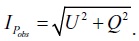
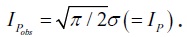
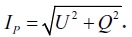
In this Section, I discuss the Ricean bias in the polar-ization intensity and suggest a new correction method. The linearly polarized intensity is obtained from Stokes parameters U and Q according to
It follows a Ricean distribution (Vinokur 1965):
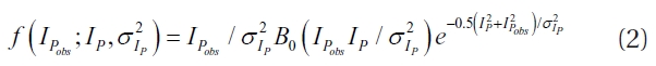
where
In the other case,
The reason is that the Rayleigh distri-bution is an asymmetric distribution. This has become known as the Ricean bias in the literature, and is caused by the positivity of the noise in
Different from the polarized intensity, the distribution function of the polarization angles remains symmetric, and no Ricean bias correction is needed (Wardle & Kronberg 1974), since there is no positivity problem in
In practice, two solutions of the Ricean bias correction are widely used.
2.1.1 The solution of Wardle & Kronberg
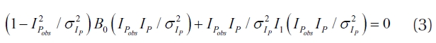
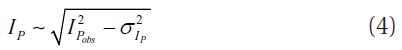
Wardle & Kronberg (1974) have suggested a solution based on the mode of the equation, namely,

A good approximation of this solution is
Conventionally,
with
is the Rayleigh distribution.
2.1.2 The solution of Killeen et al. (1986)
The other solution which is based on a more solid sta-tistical reasoning, viz. the maximum likelihood method,

was suggested by Killeen et al. (1986). With in-creasing signal-to-noise, the Maximum Likelihood esti-mate approaches the value of

A good approximation of this solution is
which is implemented in the AIPS task POLCO as such.
2.1.3 Pros and cons of the solutions
The performance of the maximum likelihood estima-tion is better at high signal-to-noise,
signal-to-noise. On the contrary, the difference at low sig-nal-to-noise, i.e. the overestimate of the maximum like-lihood solution, is significant. As mentioned in the help tool to AIPS task POLCO, one should assume an underes-timate of up to about a factor of 2 of the noise level, due to the so-called 'magic blanking'. Therefore, if one wants to go down to a 3- σ
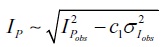
In the Wardle & Kronberg (1974) solution,
,

for a better performance in the range 3 <
Our goal is to improve the performance of the Ricean correction such that
should be reliable down to 3σ
The selection of
with
4.1 Integrated Fractional Polarization
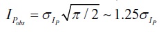
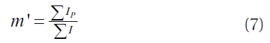
Before working out a new method to estimate the frac-tion of polarization, I discuss the integrated fractional po-larization as published in the literature, motivating this new correction method. There are two ways to estimate the fractional polarization of a region of interest. One can first integrate the polarized and the total intensity and di-vide them:
There are pros and cons to this integrated estimate. The pro is that the Ricean bias problems are largely removed by the integration. The obtained
is desirable.
In polarization studies, other important informations are the polarization angle and the RM. Since they are in-dependent of the brightness, the use of DP as obtained from

could lead to a wrong interpretation.
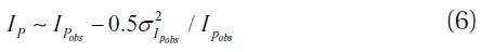
4.2 Underestimates of σIp in the Literature
In this subsection, I discuss the propagation of the sys-tematic error as due to the insufficient Ricean bias cor-rection in published DP maps. The discussion is based on the solution of Killeen et al. (1986). For the solution of Wardle & Kronberg (1974), this should be interpreted in an opposite sense. In that case, the systematic error in regions with low polarization intensity is less important, unless the signal-to-noise is too low in the absence of any σ
I consider the problem of underestimating σ
In depolarization studies, the integrated DP is rather in-dependent of the polarized and total intensity, but rather depends on
where S is the projected surface. The first case (resolved source) overestimates DP, while the second (unresolved source) underestimates it. Let us discuss this in the light of the Laing-Garrington effect. If one can assume that the jet side is brighter and more po-larized, the two arguments will be more important for the counter-jet lobe. In the first case, the Laing-Garrington effect will be emphasized through the overestimate of DP, whereas it will be reduced in the second case because of the under-estimation.
One more word of caution seems to be necessary re-garding DP structures. Patchy distributions of DP in re-gions with low


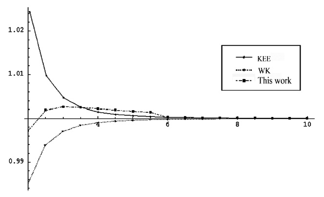
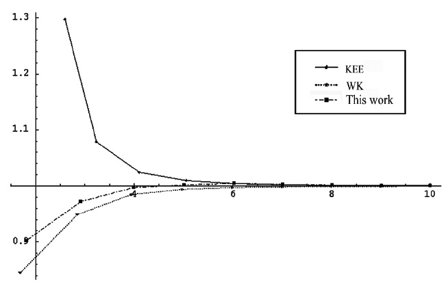
![The simulation shows the case σIp = 2σIpobs. A underestimate of σ by a factor of 2 of σIp could be possible due to the blanked values (AIPS cookbook [National Radio Astronomical Observatory 2011] see also AIPS HELP). In view of the underestimate of σIp our new solution is the best one. The solution implemented into AIPS task POLCO Killeen et al. (1986) strongly overestimates the polarization intensity while the Wardle & Kronberg (1974) solution underestimates it. The difference is much larger than that to our solution visible in Fig. 3.](http://oak.go.kr/repository/journal/11230/OJOOBS_2011_v28n4_267_f004.jpg)