Earth observation satellites require image validation and calibration procedures not only at the initial opera-tion but also regularly since the image quality in actual situations is difficult to verify before the launching be-cause of the pointing error in the space environment and the damage in the launching process. Accurate valida-tion is required for the calibration, and a validation and calibration ground site that is sufficiently bright, uniform and stable is needed for the validation. In some cases, ar-tificial structures such as a runway or road are used for the validation. However, a ground site has the drawbacks that it is affected by atmospheric and meteorological phenomena, that it involves expenses for the establish-ment and maintenance, and that the validation should be performed during the imaging period. Hence, in this study, we performed the validation process to measure image quality by observing stars. Properties of stars are already known well. Stars can be considered as ideal point light sources, and their signal to noise ratio (SNR) is large. Their along and across point spread function can be measured simultaneously. Additionally, the effects of the atmosphere, season and meteorological phenomena are negligible. Yaw steering is generally performed for the observation of the earth in order to eliminate the effects of the Earth's rotation, but the process can be neglected in the observation of stars, thus excluding the effects that decrease the image quality.
Generally, the image quality of a satellite can be known by analyzing the characteristics of the modulation trans-fer function of the point light source (Schowengerdt et al.1985, L?ger et al. 1994, 2004, Rangaswamy 2003, Zanoni et al. 2004, Yu 2011). For the IKONOS satellite, which is an Earth observation satellite, the image validation and calibration process was performed using stars. In Bowen's (2002) study, he converted irradiance into radiance, and selected 11 stars appropriate to the multispectral region using the spectral information of stars and the relative spectral response of payloads. The Gunn & Stryker spec-trophotometric information used for IKONOS contained the spectral information of 175 stars in the visible light region (Gunn & Stryker 1983). Space Imaging observed the Hyades star cluster using IKONOS, measured and cal-culated the average of the two-dimensional modulation transfer functions using six stars for panchromatic imag-es and two stars for multispectral images (Bowen & Dial 2002). In addition, a study was conducted on the radio-metric calibration and geometric calibration using stars (Kim et al. 2009). Radiometric calibration using the moon was also conducted with respect to MODIS, the payload on Terra and Aqua (Butler 2003). ITT published the results of the validation performed with various subjects on the ground and in the space using IKONOS, reporting the method to utilize each of the subjects as well as their pros and cons (Bowen et al. 2009).
In Korea, a pre-launch validation and calibration review was performed for the KOMPSAT-2 (Lee et al. 2006b). Unlike KOMPSAT-1, the importance of validation and calibration came to the fore since factors that are re-lated only with 1 m class high resolution satellite images were involved in KOMPSAT-2. For this, a site for the vali-dation and calibration was established using waterproof tarp, Siemens and lamps, and spatial, radiometric and geometric calibrations were performed on it (Lee et al. 2007, 2008a, b). The validation and calibration process of the same concept is currently prepared for KOMPSAT-3 since it employs the type of camera that is similar to that of KOMPSAT-2 (Lee et al. 2006a). Different from KOMP-SAT-2, KOMPSAT-3 has mobility in the attitude control and thus it allows a free imaging mode of which application enables to observe stars. Additionally, since KOMP-SAT-3 has a higher resolution than that of KOMPSAT-2, it is more influenced by the atmospheric conditions and the weather, but the validation and calibration based on star observation eliminates such uncertainties. For this, Kim et al. (2007) investigated the conceptual method of operation to calculate the modulation transfer functions as well as the effects of performing the observation while using the time-delay integration (TDI) on the modulation transfer functions, and verified the spectral types of the stars employed in Korea. However, appropriate stars need to be selected to performed star observation by the vali-dation and calibration method that considers the specifi-cations of the payloads on KOMPSAT-3. Thus, this article introduces the methods to select the stars by means of payload modeling as well as the scene area chosen by the method.
The objective of this study was to select the stars ap-propriate to the validation of the image quality of Korean optical remote sensing satellites using TDI. For this, we developed the process to select appropriate stars con-sidering the specifications of the satellite payloads. The brightness of a star is an important issue to the earth observation satellites since their camera has a short ex-posure time and a narrow field of view of a pixel. Thus, stars that are as bright as possible within the range where saturation does not occur should be selected considering the specifications of the payloads. The standards to select the appropriate stars were set through the modeling of the payloads. Since the spectrum information of all the stars may not be known, the relation between V magni-tude and the radiance incident to the satellite payload ap-erture is derived through the some of the existing stellar spectrums. The relation between the stellar characteris-tics and the star spectral types was derived, and the ap-propriate standards to select the stars were established. On the basis of these, general stars could be selected and the number of observable stars could be increased. The celestial bodies that are effective to the validation were selected from the given list of the stars.
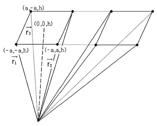
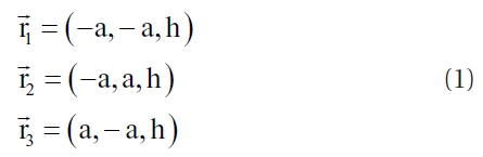
A detector of an optical payload consists of the pan-chromatic channel where black and white images can be obtained and the multi spectral channel where blue, green, red and infrared images can be obtained. The ground sample distance (GSD) was assumed to be 0.7 m for the panchromatic channel and 2.8 m for the multi spectral channel, and the standard scene size was as-sumed to be 15 km × 15 km. This study was focused on the panchromatic channel that deals with black and white images. The instantaneous field of view (IFOV) is defined as the angle through which a pixel of a charge-coupled device (CCD) can be seen by an instantaneous exposure. IFOV is expressed as angle and it is a quantity that is in-dependent on the altitude but dependent on the focal length and the pixel size. Hence, we assumed that all the pixels are square and all the IFOVs are equal. GSD holds the concept of the observation distance when a payload observes to the nadir direction of the earth. It is varied if the pixel is not oriented to the nadir direction. The IFOV of a pixel was calculated on the basis of the information that the GSD is 0.7 m when observing to the nadir direc-tion (Joseph 2000). Assuming that the altitude (h), which is the distance between the payload and the ground sur- face, is 685 km and defining the GSD, which is 0.7 m as 2 × a, а becomes 0.35 m, which is half of a projected length on the ground through a pixel. The three vectors in Fig. 1, r1, r2 and r3 are defined as in the following Eq. (1):
The horizontal IFOV (IFOVx) and the vertical IFOV (IFOVy) of a pixel can be calculated through the cross products of two vectors in Eq. (1) as shown in the following Eq. (2):
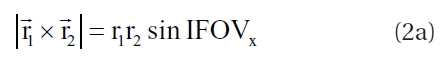
The calculation shows that IFOVx and IFOVy are the same value which is 1.0217 × 10⁻⁶ rad.
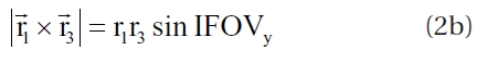
Now, a pyramidal solid angle held by a pixel is formed, and the size in the space is calculated. Substitution of defined previously Eq. (1) to Eq. (3) gives the solid angle (Oosterom & Strackee 1983):
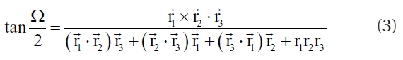
In Eq. (3), Ω denotes the pyramidal solid angle held by the three vectors. The pyramidal solid angle can be cal-culated by substituting the three vectors and doubling it. Summarization of it gives the solid angle, Ψ, as in the fol-lowing Eq. (4):

where Ψ means the solid angle in which the pyramidal space is expressed on the celestial sphere. The unit for solid angle is steradian (sr), and the sum of solid angle in all space is 4π sr. Substitution of a and h to Eq. (4) gives the solid angle held by a pixel, which is 1.0439 × 10⁻¹² sr.
In order to apply TDI to a payload, the effect of moving on the ground track while observing a star should be re-produced. There are 64 linear CCDs in the panchromatic channel to the direction in which the satellite moves. It is assumed that the number of TDI can be chosen among 1, 8, 32 and 64. Choosing '64' means that 64 images that can be acquired by one linear CCD are superposed. The number of lines passed through in a second by the image on the CCD to the direction in which the satellite moves in the CCD coordinates is called line rate. Another impor-tant variable is the exposure time, because saturation, which is a characteristic of a CCD, should be prevented. In the saturation state, the digit number is not increased anymore even when receiving light. Validation and cali-bration should not be performed with respect to the stars where saturation occurs. Thus, suitable star brightness needs to be selected according to the exposure time. If TDI is used, the exposure time (texposure) is dependent on the TDI number and the line rate. Their relation is expressed as in Eq. (5):
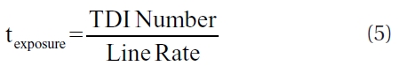
As the TDI number is increased, the number of linear CCDs used for the observation is increased. Thus, the im-age should pass through all the lines used on the CCDs and thereby the exposure time is increased. As a result, the line rate is increased and the rate to scan the ground or the celestial sphere is increased, reducing the time to be exposed to the observation target. Since the appro-priate star brightness is dependent on the TDI number and the line rate, the exposure time is taken into account when selecting stars.
Image validation requires the selection of stars that do not exceed the saturation state of optical payloads and that are easily distinguished from noise. For this, the specifications of the payloads and the brightness of stars should be known. Brightness of light at the aperture is defined differently for the stars that are extended tar-gets and point sources (Bowen 2002). Payloads of earth observation satellites have the specification for extended targets. The brightness of extended targets is defined as radiance having the unit of W/cm2sr. The unit of extended targets includes solid angle, projected source area, and light energy incident in unit time (W). On the other hand, the brightness of point sources is defined as irradiance having the unit of W/cm2. Since point source is incident to a single point, not to a unit space, the brightness is de-fined as irradiance. Hence, it is necessary to convert the brightness of point sources given as irradiance to radi-ance. Firstly, the procedure to obtain irradiance of stars was carried out.
The Gunn & Stryker stars (Gunn & Stryker 1983) of the STSCI database were used in this study. The database pro-vides data in 10 A interval in the range of 3,180 ~5,750 A and in 20 A interval in the range of 5,780~ 10,560 A. Irradi-ance is provided in the unit of 'Pho-tlam' which is Photons/cm2 secA for spectral irradiance. Thus, number of photons need to be converted to energy unit using Eq. (6):
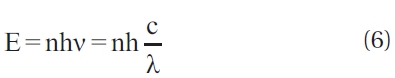
Substituting the number of photons (n), speed of light (c), Plank's constant (h) and respective wavelengths (λ) and converting A to ㎛, the spectral irradiance was obtained in W/cm2㎛ unit, and the result was consistent with that of Bowen (2002). The spectral radiance was ob-tained by integrating given information, Eq. (4). The solid angle of one pyramidal pixel was calculated using Eq. (4). Assuming the ideal case where all light from a star comes onto one pixel, the spectral radiance could be calculated
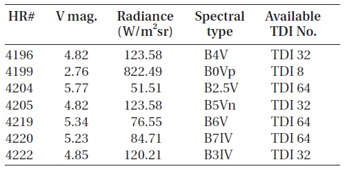
[Table 1.] Selected stars from Gunn & Stryker (1983).
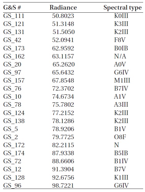
Selected stars from Gunn & Stryker (1983).
by dividing with the solid angle of a pixel.
Relative spectral response of the satellite should be considered in order take the saturation of image payloads into consideration. However, in this study, we assumed that the relative spectral response of black and white im-age is uniform in the range between 450 and 900 nm in order to simplify selection of stars. We assumed that the saturated radiance is 100 when the TDI number is 64 and the line rate is 9,700 Hz. In this article, the unit for radi-ance is W/m2sr. We also assumed that signals can be well distinguished without being affected by noise if a star has the radiance of 25 or greater. Considering the solid angle of payloads in the Gunn & Stryker stars (Gunn & Stryker 1983), spectral irradiance was converted to spectral radi-ance. Twenty two stars of which radiance was between 50 and 100 were found in the visible light region, 450~900 nm. Table 1 shows the list of the selected stars.
In general, selection of stars is limited because no spectral information is provided for a number of stars. The Gunn & Stryker star list provides information about 175 stars. Using the spectral types provided by the list, we investigated the method to find appropriate stars on the basis of the assumption that stars of the same spec-tral type have the same spectral energy distribution. The spectral energy distribution was assumed to be a func-tion of temperature. If the selected scene area is an open cluster where the evolution type of stars is similar with each other, the difference due to the evolution type may be minimized. Hence, if the spectral type is equal, the temperature range may be similar. Additionally, if the elements of the stars are ignored, they will have a simi-lar spectral energy distribution depending only on the temperature according to the Plank's law. This method provides the methodology to select stars and gives the advantage of allowing selection of quantified stars. Appli-cation of detailed spectral types may provide a better out-come, but it is difficult because there are not many stars in each detailed spectral type for the number of stars is limited to 175. If the V magnitudes of stars are n and m, and their flux is fn and fm, the general relation between the magnitude and flux is as in the following Eq. (7) (Zeilik & Gregory 1998):
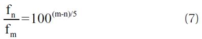
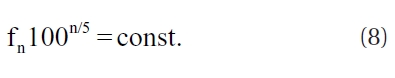
If a star of the magnitude of m is considered as a stan-dard star, the m magnitude and the flux (fm) are found as well-known constants as in Eq. (8):
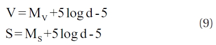
Distance modulus can be described with the V fil-ter viewing magnitude (V) and the absolute magnitude (MV) as in Eq. (9) (Zeilik & Gregory 1998), and S, which is the filter magnitude of a satellite optical pay-load, can be defined in the same form. The filter of the optical payload is a filter that has a uniform response in the range of 450~900 nm described previously. In Eq. (9), d denotes the distance from the earth to the star.
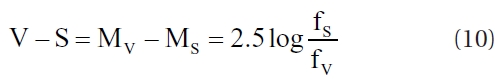
With respect to the V and S filters of a star, the effect of distance on brightness can be eliminated by subtract-ing the two equations in Eq. (9). With the result, Eq. (10) can be derived through the relation between V magnitude and flux in Eq. (7):
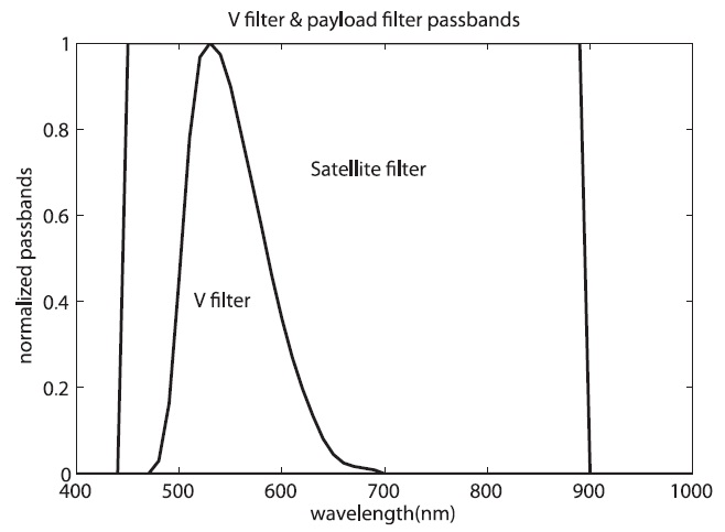
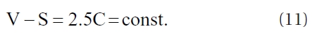
As shown Fig. 2, the V filter and the filter of the satel-lite image payload may be considered to have a similar frequency response in visible light bandwidth. Once the spectral type of a star is given, the spectral energy distri-bution becomes similar and the magnitude difference of the two filters can be assumed to be constant. The mag-nitude difference can be expressed as the constant as shown in Eq. (11). The spectral intensity may be depen-dent on the elements, mass, radius, distance to the earth and the evolution type of a star, but the flux difference of the light that has passed through each of the filters should be constant if the temperature is constant.
Using Eq. (10) and Eq. (11), the flux of the V filter and the payload filter can be summarized as in Eq. (12):
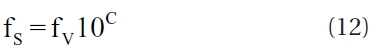
Since C is a constant, the flux that has passed through the V filter and the flux that passed through the payload filter are in a linear relation. Substituting the flux of the V filter to Eq. (8) gives the relation between the V magnitude and the flux that has passed through the satellite filter as in Eq. (13):
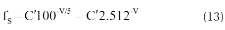
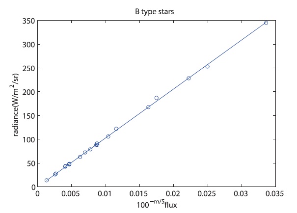
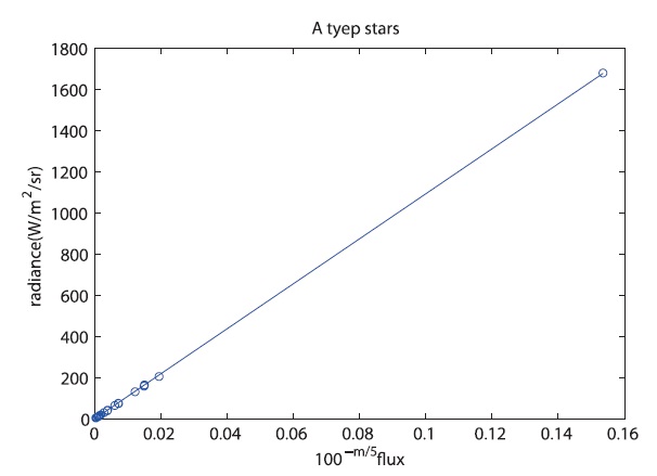
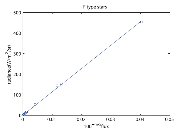
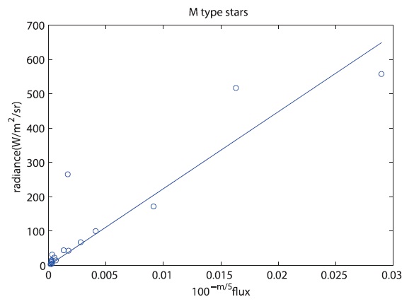
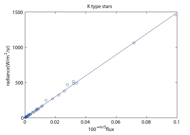
Under the condition that the absolute magnitude dif-ference between the V filter and the payload filter shar-ing a similar observation band is constant if the spectral type is the same, the flux at the aperture can be calculated with the V magnitude. The flux can be considered as the irradiance that has passed through the payload aperture and detected. Dividing the irradiance with the solid angle of a unit pixel gives the radiance. The coefficient (C´) is determined by the least squares method based on the re-lation between the flux and the V magnitude that can be calculated from the Gunn & Stryker stars (1983). Applica-tion of the determined coefficient to general stars of the same spectral type enables to predict the flux on the basis of the V magnitude.
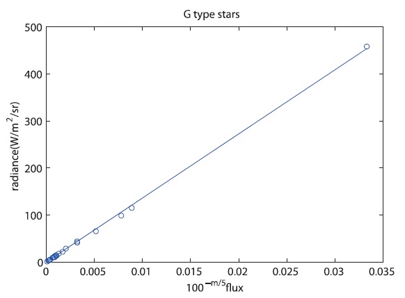
In the Gunn & Stryker star list, stars of the spectral type O are rare, and Type M stars have small linear fac-tors. Other stars of Types B, A, F, G and K have the propor-tionality between the flux at the payload aperture and the flux of the V filter and their coefficients are different with each other. Figs. 3-8 show the relations between the flux that has passed the satellite payload and the V magnitude in the respective spectral types. This method is based on the assumption that stars of the same spectral type have a similar spectral energy distribution. In other word, the spectral types should be divided in more details, it is dif-ficult since there are not many stars included in the Gunn & Stryker star list. In addition, the irradiance of stars of each spectral type is not distributed uniformly, and thus the precision of the least squares method may be low. Be-cause the irradiance was derived on the basis of the as-sumption that the relative spectral response in the band where input is allowed is constant, the relative spectral response of the payload needs to be taken into account in order to acquire a more precise value. Nevertheless, ap-plication of the previous results enables to estimate the irradiance of a star in the case where the V magnitude and the spectral type of the star are known.
Since it is good to have more candidate stars for the validation of satellite optical payloads, stars were select-ed in addition to the Gunn & Stryker stars. The list of the stars used was from the Yale Bright Star Catalogue 5th edi-tion (Hoffleit et al. 1991). This star list provides informa-tion about 9,110 celestial bodies that are relatively bright within the magnitude of 6.5, including the right ascen-sion (RA), declination (DEC) in J2000 coordinate, bright-ness and spectral type. The radiance to be detected after passing through the payloads could be calculated for all the stars in the Yale Bright Star Catalogue.
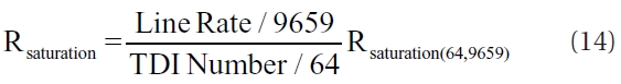
As the TDI number is decreased, the exposure time is shortened, as in Eq. (5), and thus a brighter star should be observed and the saturation occurs at a higher radi-ance. As the line rate is reduced, the exposure time is proportionally increased and thus a darker star may be observed. However, the saturation may occur in a rela-tively dark star. Validation and calibration should not be performed with respect to the stars where saturation oc-curs. It was assumed that the equivalent saturation radi-ance is 100 if the TDI number is 64 and the line rate is 9,659 line/sec, and the value was defined as Rsaturation(64, 9659). Then, the equivalent saturation radiance depending on the TDI number and the line rate, Rsaturation, can be calcu-lated as in Eq. (14):
In case of SNR, as the TDI number is reduced to the half, the exposure time is also reduced to the half and thereby the SNR equivalent radiance is increased and the SNR is increased by

times due to the feature of the TDI technique. This may increase the SNR as exposing to the TDI number of linear CCDs and using the values ob-served at each stage (Wong et al. 1992).
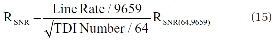
Similarly, the SNR equivalent radiance at which the signal and noise can be sufficiently distinguished was de-fined as RSNR and the value was set to be 25 if the TDI num-ber is 64 and the line rate is 9,659 line/sec. It was assumed that the signal and noise are not easily distinguished if the light incident to the payload has the radiance lower than the SNR equivalent radiance and the light has the SNR greater than 100 in the opposite case. Then, the SNR equivalent radiance depending on the TDI number and the line rate can be calculated as in Eq. (15):
The maximum radiance was set to be 90% of the equiv-alent saturation radiance whereas the minimum radiance was set to be 60% of the equivalent saturation radiance. Thus, stars that are brighter than the minimum radiance and darker than the maximum radiance may be selected from the Yale Bright Star Catalogue.
Assuming that TDI numbers can be selected among 64, 32, 8 and 1, observation can be performed using each of the TDI numbers. In that case, as the TDI number is in-creased, the exposure time is increased and thereby the radiance proportional to the energy received in a unit time should be decreased. Another thing that should be noted when selecting stars is the SNR. According to above, the SNR is increased in proportion to the square root of the TDI number, if the TDI number is increased. On the other hand, the SNR is decreased as the TDI num-ber is decreased. Hence, the SNR equivalent radiance is not directly proportional to the exposure time. If the TDI number is increased, the exposure time is increased so that a darker light source may be observed. The SNR is in-creased in proportion to the square root of the TDI num-ber, which is an advantage of TDI.
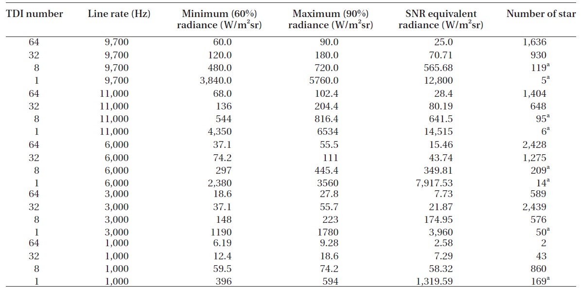
Previously, we assumed the equivalent saturation ra-diance and the SNR equivalent radiance when the TDI number is 64 and the line rate is 9700 line/sec. We also set the radiance range where the signal and noise can be distinguished without having the saturation for being too bright, varying the line rate to 9,700 Hz, 11,000 Hz, 6,000 Hz, 3,000 Hz and 1,000 Hz. Decreased TDI number gives wider dynamic range but a smaller number of sufficient bright stars, which makes the observation difficult. In ad-dition, the SNR equivalent radiance is also increased and thereby a considerable amount of noise is included in the image. To obtain images with little noise, the TDI number may be increased or bright stars should be selected for the observation. As the line rate is decreased, the number of observable stars is increased since darker stars can be observed. However, over a certain value of line rate, the dynamic range is increased and thus the number of ob-servable stars is decreased while the SNR remains similar.
The list of stars having the radiance that is lower than Rsaturation and higher than RSNR can be obtained depending on the TDI numbers and the line rates. Table 2 shows the radiance between 90% and 60% of the saturation radiance in each situation, assuming that the TDI number and the line rate may be selected. We assumed that there is about 10% error in determining the saturation radiance and then showed the number of stars in the range. Table 2 also shows the values of the SNR equivalent radiance at which the signal is relatively well distinguished from the noise. If providthe SNR equivalent radiance is greater than the minimum radiance, the SNR equivalent radiance is used. Even if an actual star is darker than the minimum radiance, it can be observed if it is brighter than the SNR equivalent radi-ance. The cases where there are some stars darker than that or where all the stars are dark are marked as 'a'.
It is required to select an appropriate scene area on the basis of the given observed star list and to identify the stars that can be applied to the image validation among the stars in the scene area. The FOV was assumed to be 1.42 degree, and the area where the greatest number of stars was included in the view of the optical payloads was selected as the scene area. The area where stars of vari-ous brightness values were included was preferred. We excluded the area where there is a nebula of which point spread function is hard to analyze, the area of which point spread function is not easily identified for containing many superimposed stars, such as a globular cluster, and the area of which point sources are affected by multiple stars such as binary stars. With respect to the selected scene areas, the distribution of stars was verified in the viewing area. When compared with other astronomical programs, a considerable number of stars showed a simi-lar distribution, indicating that the position of star was accurate in the selected scene areas, although few stars were included in different star lists. Among the scenes that satisfied the abovementioned conditions at each magni-tude, we selected three areas that were most appropriate

TDI number can be chose for 1 8 32 64 and the number of stars is represented in that 60% to 90% of saturation equivalent radiance whether line rate could be chose for 9700 11000 6000 3000 1000 Hz.
for image validation. The three selected areas, which are the samples to explain the method of selecting stars, are close to open clusters and they include the maximum number of stars that have a similar evolution and are suf-ficiently bright. The stars were named with the Harvard Revised numbers. The list of the stars included the TDI numbers that are observable at the line rate of 9,659 Hz. The SNR was not taken into consideration. Available TDI numbers that are smaller than the saturation radiance of the TDI number were selected
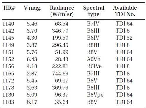
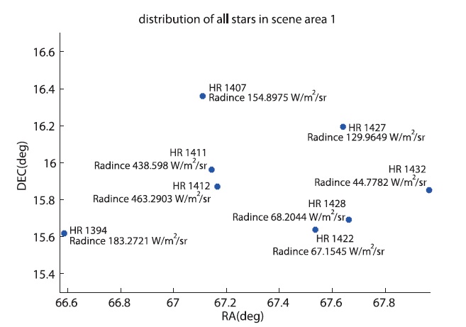
Scene Area 1 is a part of an open cluster in Taurus. Eight of the stars in the list are included in the scene area. The observation is convenient because bright stars within 1.5 of magnitude such as Aldebaran, Capella and Rigel are lo-cated nearby. The center of the scene area is at RA 67.2708 degree (4:29:05) and DEC 16.0000 degree (+16:00:00). Table 3 is the list of stars included in Scene Area 1. Fig. 9 is shows the distribution of the Yale Bright stars included in Scene Area 1 as output by the developed software.
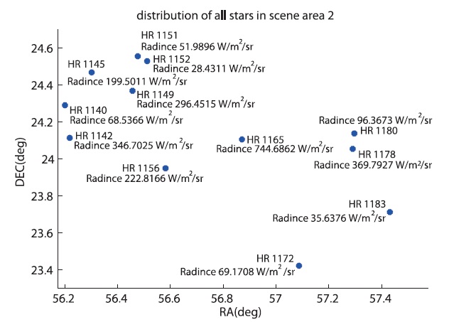
Scene Area 2 is a part of the Pleiades open cluster and it includes 12 bright stars. Stars of various magnitudes be-tween 2.5 and 6 are distributed in Scene Area 2, provid-
ing various point light sources needed for image valida-tion. The observation is convenient because bright stars within 1.5 of magnitude such as Aldebaran and Capella are located nearby. Scene Area 2 includes more stars than those of Scene Area 1. The center of the scene area is at RA 56.8750 degree (3:27:30) and DEC 24.0000 degree (+24:00:00). Table 4 is the list of stars included in Scene Area 2. Fig. 10 is shows the distribution of the Yale Bright stars included in Scene Area 2 as output by the developed software.
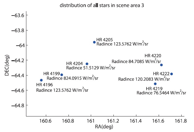
Scene Area 3 is a part of the IC2602 open cluster and it includes 7 bright stars. The observation is convenient be-
[Table 3.] Stars in selected scene area 1.

Stars in selected scene area 1.
[Table 4.] Stars in selected scene area 2.

Stars in selected scene area 2.
[Table 5.] Stars in selected scene area 3.

Stars in selected scene area 3.
cause Canopus of the magnitude of -7.2 is located near-by. The center of the scene area is at RA 161.1250 degree (10:44:30) and DEC 64.2489 degree (-64:14:56). Table 5 is the list of stars included in Scene Area 3. Fig. 11 is shows
the distribution of the Yale Bright stars included in Scene Area 3 as output by the developed software.
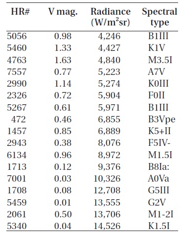
In Scene Areas 1, 2 and 3, most of the stars can be ob-served at the TDI numbers of 64, 32 and 8. If the TDI num-ber is 1, a single bright star should be observed because there are not many bright stars and thus two or more bright stars can be hardly included in an image. Table 6 shows the list of the 17 stars with the brightness higher than the radiance of 4,200. The stars to be observed can be selected among the stars in Table 6, considering the radiance according to the line rate.
[Table 6.] The selected brightest stars in Yale Bright Star Catalog.

The selected brightest stars in Yale Bright Star Catalog.
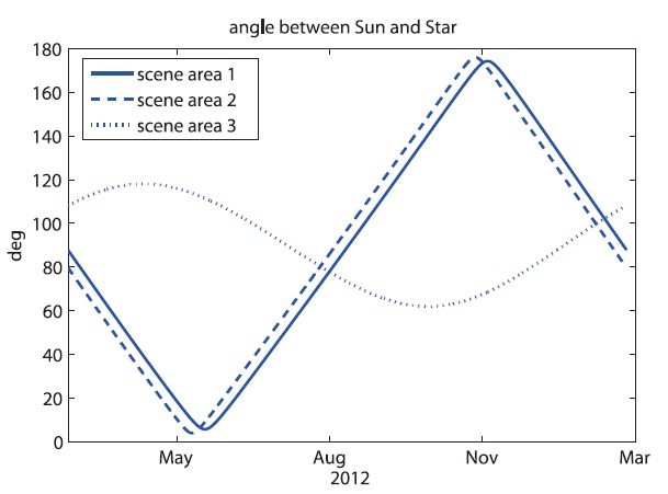
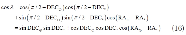
Even in the selected Scene Areas 1, 2 and 3, stars can-not be observed if the star is close to the sun since the solar light is incident to the optical aperture. The sun only moves within ±23.5 degree of the DEC which is the slope of the ecliptic plane in the J2000 coordinates. Since the DEC of Scene Areas 1 and 2 is within 43.5 degree, they may be located close to the sun. On the contrary, the DEC of Scene Area 3 is -64.2489 degree, at least 40 degree far from the sun, and thus observation is possible anytime in a year regardless of the position of the sun. In order to cal-culate the solar position at a time, the solar position, RA⊙ and DEC⊙ should be known in the J2000 coordinates cen-tered on the earth. For this, we employed the algorithm to calculate the solar position information developed by the National Renewable Energy Laboratory (Reda & Andreas 2008). Considering the solar position calculated by the al-gorithm and the positions of the selected Scene Areas 1, 2 or 3 (RA*, DEC*), the relative angle between the sun and the star can be calculated through spherical trigonom-etry. Eq. (16) shows how the function of the relative an-gular distance between the center of a scene area and the center of the sun can be obtained using the cosine rule of spherical trigonometry:
We calculated the relative angles between the sun and the Scene Areas 1, 2 and 3 over one year from March 1, 2012. Fig. 12 shows the angles between the sun and the Scene Areas 1, 2 and 3. It is expected that the observa-tion may not be allowed between May 9 and June 18 in 2012 in Scene Area 1 and between April 30 and June 10 in 2012 in Scene Area 2 when the relative angles were within 20 degree. On the contrary, there is no time period when Scene Area 3 approaches the sun within 60 degree. All-time observation is possible in Scene Area 3, being free from the effect of the sun, but the observation is only pos-sible when the TDI number is 32 or 64. Since there are only three stars that are appropriate for observation for each TDI number, Scene Areas 1 and 2 may be used when a greater number of stars is required or when the observa-tion needs to be performed at the TDI of 8.
In this study, we developed a program for the selec-tion of appropriate stars so that earth observation satellite Prousing TDI can perform image validation while perform-ing observation of stars. Appropriate stars were selected from the 175 Gunn & Stryker stars according to the given spectrum. We also performed additional work to increase the number of apptopriate stars that may be selected. As-suming that stars of the same spectral type share similar temperatures, based on the Gunn & Stryker star list, we calculated the relation between the stellar magnitude and the radiance of the light that has passed through the satellite optical payloads. The relation was derived on the basis of the assumption that the relative spectral response of the payloads is constant in the visible light region. We also selected stars appropriate for the observation among about 9000 stars in the Yale Bright Star Catalogue 5th edi-tion. Relatively bright stars that are easily distinguished from the noise were selected in the range where no satu-ration occurs, considering the saturation state of the pay-loads. We also developed the software that provides the list of the selected, observable stars and visualizes their distribution when the scene area is determined accord-ing to the FOV of the satellite. Additionally, we proposed observation in three scenic areas where there are many stars in the viewing angle of an image. The period of time when observation is possible was also calculated consid-ering the solar effect. When performing observation in a scene area with a certain TDI number, the application of the method to acquire one point spread function from several stars will provide the advantage of increasing the number of samples. When applying this method, using 3 to 6 stars may be appropriate, even though the method may depend on the relative position of the center of sev-eral stars in the pixel. The result of this study may be used to verify the performance of the optical payloads of Ko-rean satellites.