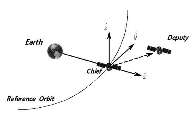
Satellite formation flying is defined as a set of more than one satellite whose states are coupled through a common control law (Scharf et al. 2004). Formation flying missions can be divided into two main categories, based on the motion of the chief satellite, which is a reference point to describe a relative motion. First, for the case of a circular reference orbit, formation flying can be applica-ble to Earth observation, including space interferometry,and synthetic apertures. The second main category is for the case of an eccentric reference orbit, which has several advantages in scientific missions, such as the magneto-spheric multiscale (MMS) mission (Curtis 2000, Curtis et al. 2003) and the cluster II mission (Dow et al. 2004). To meet the scientific mission goals, four-spacecraft forma-tions are commonly used to take measurements in three dimensions at intersatellite distances on the order of sev-eral kilometers. The work presented in this paper was mo-tivated by the need for an algorithm that can provide ini-tial conditions for formation flying at the beginning of the region of interest to maximize scientific mission goals for the case of a tetrahedron formation with relatively high eccentricities, such as an MMS mission. Recently, several papers have attempted to solve tetrahedral formation op-timization problems similar to the one considered in this paper by focusing on various ways to calculate trajecto-ries and determine initial conditions at the beginning of a region of interest. Huntington & Rao (2008) designed a minimum-fuel trajectory to transfer four spacecraft from a degraded tetrahedral formation into a tetrahedron that satisfied certain geometric quality constraints for a por-tion of its orbit. Guzman (2003) developed a general op-timization procedure for tetrahedron formation control to calculate the maneuver sequence that minimizes the fuel needed to transfer the formation from its current configuration to the target configuration. Chavez Clem-ente& Atkins (2005) developed hierarchical optimization schemes. Zanon & Campbell (2005) presented a search space reduction technique to solve the coupled guidance and control problem. Hughes (2008) found optimal orbit states for MMS and laser interferometer space antenna mission (LISA Project Office 2000) by using a direct tran-scription method. To take into account the actual size of the tetrahedron, Hughes (2008) proposed a polynomial function and adopted a performance metric that evalu-ates both the size and the shape of a tetrahedron. Except for Hughes (2008), these works assume an active con-trol to reconfigure the formation. Unlike the works cited above, we do not consider reconfiguration maneuver be-tween different phases, but coast phase with a periodic-ity condition; however, no maneuvers are allowed in the coast phase, and several constraints are applied only in this region. Also, a quality factor is adopted as a cost func-tion, and relative states are considered to make it easier to determine the configuration of the tetrahedron in the region of interest.
Optimal initial conditions determined in this work make it possible to estimate the configuration of tetrahe-dron formation and final states at the end of the region of interest phase, which can be used for reconfiguration maneuver and fuel balancing.
2. RELATIVE DYNAMICS IN AN ELLIPTICAL REF-ERENCE ORBIT
For tetrahedron formations, the satellites are moving in an elliptical orbit. Hence, we should use the Tschauner-Hempel equations, which were first derived by Tschauner & Hempel (1965), as follows.
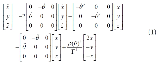
where
upper dot represents the differentiation with respect to time
Changing the independent variable from time (
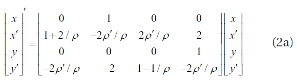
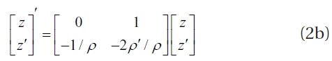
where primer (
where

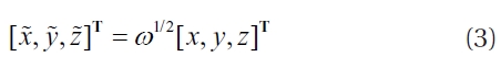
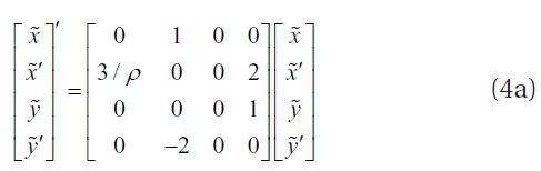
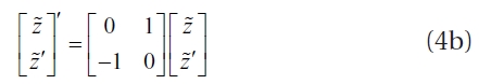
the orbital rate of the Chief satellite. With the same procedure as that derived by Humi (1993), Eqs. (2a) and (2b) become very simple:
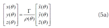
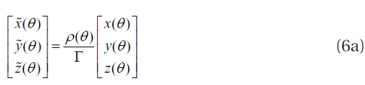
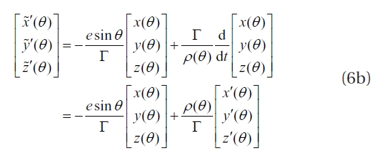
It is important to note that the actual position (

are related to the pseudo-position

and pseudo-velocity

as follows:
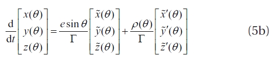
or
In this paper, we assumed the MMS-type mission to determine the initial conditions of tetrahedral forma-tion. For MMS, to achieve a fundamental advancement in our understanding of the Earth's magnetosphere and its dynamic interaction with the solar wind, a four-spacecraft formation has to be a near regular tetrahedron formation, within a region defined by ±20 deg in true anomaly about the orbit apogee. Also, in the region of interest, the absence of maneuvers benefits the gathering of scientific data by limiting the orbital disturbances. Consequently, the thrust is zero in the region of interest. Although no maneuvers are allowed in the region of interest phase, several constraints on the formation are applied in the region of interest. To determine the quality of the formation, we adopted a performance metric that evaluates the shape of a tetrahedron consisting of the actual volume and the average side length. In addition to minimizing the cost function, periodic conditions at the beginning of the region of interest were adopted as boundary conditions to form optimal conditions in the next measurement phase in the region of interest.
The problem can be formulated to determine state variables
(
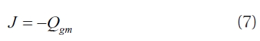
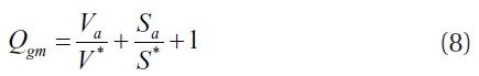
where, Qgm is a quality factor defined by Eq. (8).
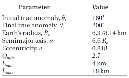
The boundary conditions are given by Eqs. (13 and 14) and Eq. (16). Dynamic constraints are set as Eq. (2). For MMS mission, the region of interest is fixed (160? <
As the formation shifts in the region of interest, it must maintain a certain geometry to take useful scientific mea-surements. In particular, the two important aspects to the formation geometry are the shape and size of the forma-tion. The most common metrics, typically called quality factors, are the Glassmeier parameter (Robert et al. 1998) defined by Eq. (8), which compares the volume and sur-face area of a tetrahedron with that of a regular tetrahe-dron of the same average leg length.
where
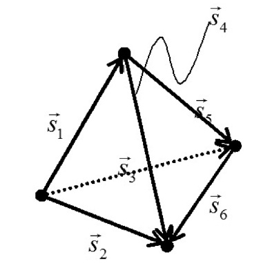
If we assume one of the spacecraft is the reference, then there are three relative position vectors that describe the relative geometry of the spacecraft, and we will define them as

and

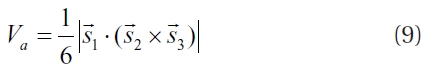
The vector

and

depicted in Fig. 2 are used to compute the surface area in Eq. (10). Knowing these quantities, we can calculate the volume of the tetrahedron using
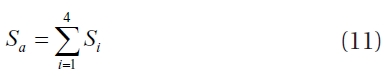
The surface area of the actual tetrahedron is computed as follows. First, let
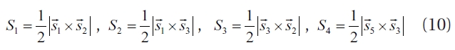
Then, the surface area of the actual tetrahedron is given as
The average side length
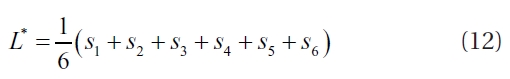
where si (
The ideal geometry for this mission is a regular tetra-hedron with 10 km spacing between each satellite, but in-vestigators have noted that there is considerable flexibil-ity here (Hughes 2004). In particular, the acceptable value of
Note that the Glassmeier metric is insensitive to the size of the tetrahedron, meaning an additional constraint is required to constrain the size of the tetrahedron. Al-though an average interspacecraft separation of 10 km is considered ideal, acceptable science return is still pos-sible for average separations ranging from 4 to 18 km (Hughes 2004). Hence, the following path constraint is enforced during the region of interest that bounds the av-erage side length
In addition to the aforementioned path constraints, we must satisfy periodicity conditions to have the spacecraft returning to the initial relative states. In a previous study, Sengupta & Vadali (2007) found the necessary conditions on the initial states that produce periodic solutions at an arbitrary true anomaly as follows.
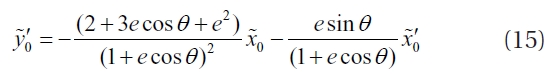
Also, Eq. (15) can be rearranged using the actual position (
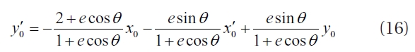
The numerical solutions are obtained by a general pur-pose optimization code: the Sparse Optimal Control Soft-ware (SOCS) (Betts & Huffman 2005) using the numerical values for the parameters shown in Table 1 and the nu-merical values for the initial guesses of each satellite as follows.
where
SOCS solves optimal control problems using a direct transcription method by which the dynamic system (Eq. 4) is converted into a problem with a finite set of vari-ables. The discretization scheme used in this paper is the second order trapezoidal method. This method produces a distinct set of nonlinear programming variables. Also, SOCS utilizes the mesh refinement algorithm to improve the accuracy of the discretization. The solutions are then determined using sequential quadratic programming.
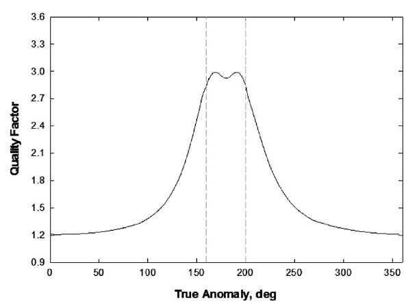
Recall that the primary mission goal for the case of MMS we consider is to maximize the quality factor given by Eq. (8), in the region between 160 and 200 deg true anomaly. Fig. 3 shows the quality factor during one
[Table1.] Parameters used in the optimization and simulation.

Parameters used in the optimization and simulation.
orbital period. We can see that the quality factor is near 3 during the region of interest.
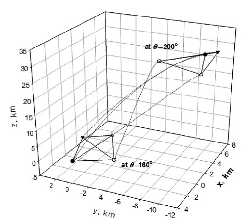
Fig. 4 shows the configuration of tetrahedron forma-tion in the region of interest. During the coast phase in the region of interest, the orientation and the size of tet-rahedron changes consistently.
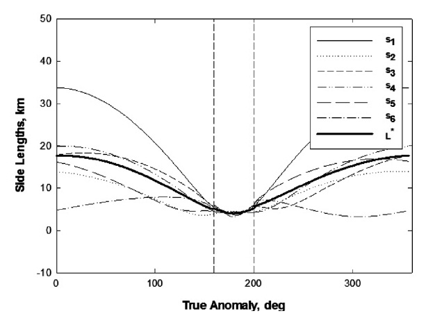
Fig. 5 shows the evolution of the six individual sides and the average side length during one orbital period. Through an inspection of the plot in Fig. 5, we can see that the average side length is in the range between 4 and 18, which is acceptable in the scientific measurements.
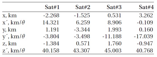
[Table 2.] Optimal initial states for MMS (at θ = 160˚).

Optimal initial states for MMS (at θ = 160˚).
Table 2 provides optimal initial relative states for MMS at the beginning of the region of interest. Initial states listed below enable scientific measurements repeatedly during the same phase without thruster maneuvering and maximize the quality factor.
In this paper, we present an algorithm that can provide initial conditions for formation flying at the beginning of a region of interest to maximize scientific mission goals for the case of a tetrahedron formation with relatively high eccentricities. Also, we found that there exist an optimal configuration and states of a tetrahedral satellite forma-tion. As the periodicity condition is adopted, the relative position of satellites in the tetrahedral formation can be maintained during every scientific measurement phase without any thruster maneuvering. Because it is highly nonlinear and dependent on upwards of 20 variables, it is doubtful that a truly optimal solution can be found. How-ever, finding a near-optimal solution is entirely plausible, and the evolution of quality factor we calculated shows sufficiently good performance. Hence, the optimal initial conditions determined in this work can be used to design an overall concept for reconfiguration maneuvers be-tween different phases.