The methods for the indirect observation of space objects from ground station without communication include radar, laser and optical observation. Space ob-jects refer to not only satellite under operation but also all kinds of artificial objects in the space such as decom-missioned satellites, rocket bodies and space debris. To observe such space objects, suitable observation tech-nology should be used according to the orbital charac-teristics of the target space object. The radar provides the advantage to find out the range to an object immediately, but the observation of space objects beyond a certain low earth orbit is difficult by this method. The laser facility like satellite laser ranging allows precise measurement of the range to an object, but it is difficult to survey a wide area at one time and to surveil high altitude space objects over a certain altitude. The optical technology enables to observe space objects regardless of their orbits, but only the relative angular distance information can be obtained and the objects that do not reflect the sunlight are hardly observed (Lee et al. 2004).

The optical observation is often used for the observa-tion of high altitude space objects. The optical observa-tion is not limited by the range to the observation target. The optical observation is appropriate for the observa-tion of high altitude space objects since they stay in the Earth’s shadow for a relatively short time. Most space surveillance facilities including the Ground-Based Elec-tro-Optical Deep Space Surveillance (GEODSS) perform surveillance of high altitude spaces by means of optical observation (Schildknecht 2007).

A geostationary orbit, which is useful in various areas, needs continued surveillance for the efficient utilization. A geostationary orbit is about 42,164 km far from the cen-ter of the Earth and has the ring shape extended from the Earth's equator. The space objects on the geostationary orbit always maintain fixed elevation and azimuth when viewed from a ground station. Hence, they can be used for various purposes including communication and weather observation, and production of geostationary satellites cost a considerable amount of resources. Thus, the coun-tries that operate geostationary satellites are taking many efforts to maintain and protect geostationary orbit.

Each geostationary satellite is to be operated within its own positional area, which is to prevent collision be-tween satellites and communication or broadcasting ra-dio frequency interference. Therefore, the number of geo-stationary satellites that can be launched is limited and thus each country is taking various efforts to occupy the positions favorable to their purposes. For example, the KOREASAT 1 satellite, after the mission was completed, has been rented to France for the purpose of occupying the country's own orbit. Some countries have illegally placed their own satellites on the unpermitted longitude (Gunter's Space Page, Lee et al. 2011a, c).

Station keeping is performed periodically to place geo-stationary satellites within the designated zones. For in-stance, Korea performs station keeping for the Commu-nication, Ocean and Meteorological Satellite (COMS) in the north-south direction and in the east-west direction one time per week and for the KOREASAT satellite one time per week with the ±0.05 degree zone (Lee et al. 2003, 2011b). Thus, the geostationary satellites currently in op-eration are always within the designated zones. Surveil-lance of the designate zones is the first step to surveil the objects that may collide with the satellite for the safety's sake.

The actual risk of collision between geostationary satel-lites in operation with other space objects has been iden-tified in various cases. The other space objects include space debris and decommissioned satellites. In January and February in 2011, an inclined geosynchronous satel-lite of a foreign country came into the orbit of the COMS (Lee et al. 2011a). The risk of collision between the two satellites was very high. The size of such an unidentified space object is various ranging from rocket bodies to space debris that is too small to be detected. Some are on the list of the Space Surveillance Network, but other are hardly tracked.

Currently, the number of space objects that are un-der tracking is about 15,000 according to the U.S. Stra-tegic Command including active satellites, decommis-sioned satellites and other space debris. About 1,100 of 334the tracked space objects are active satellites (Celestrak 2011). The size of space objects that can be tracked is 10~20 cm on a low earth orbit and 1 m or greater on a high altitude orbit. The space objects that are smaller than 1 m may be detected but they are not tracked continuously (Schildknecht 2007).

Follow-up observation is required to decide the risk of the unidentified space objects that have not be listed on the United States Strategic Command (USSTRATCOM) catalogue (Musci et al. 2004, Space-Track 2011). Initial orbit determination (IOD) is necessary to perform follow-up observation. However, IOD is hardly performed at the precision level of general orbit determination because the observation data for unidentified space objects are not sufficiently many. Moreover, a small number of observa-tion data are used for IOD, the observation error affect the orbit determination significantly. Hence, the positioning precision should be improved through the satellite posi-tioning method and the appropriate observation strategy for it.

The research on the space object IOD in Korea began with 'The Study on Preliminary Orbit Determination' by Kim et al. (1988). Thereafter, Lee et al. (2004) published the research results on IOD and precise orbit determina-tion using actual optical observation results. Choi et al. (2009) presented the method for the satellite position determination on the observed image, IOD and the dif-ferential correction results by means of actual optical ob-servation. Hwang & Jo (2009) compared the precision of IOD methods depending on the time spans using three different observation data and reported the differences.

Space surveillance is generally based on the indirect observation of the target space objects which is greatly different from actual operation of satellites. In particular, space objects surveillance using an optical telescope is the method that has been continuously used since hu-mans launched artificial space objects. The method is ap-plied in various research areas including the calculation of the orbit information with a precision level at which space objects can be tracked for a certain period of time and the surveillance of the distribution of space debris of small sizes.

In this study, we observed space objects with an opti-cal telescope that is used for celestial body observation and performed IOD in order to carry out the follow-up observation. For this, we firstly compared the positioning methods that are used to determine the position of satel-lites from the observed images by the optical telescope images. The observation target was the COMS, and the objective of orbit determination was to acquire the ini-tial orbital elements that can be used in the follow-up observation. Hence, the orbit determination precision was evaluated with reference to the possibility of the follow-up observation. The null-eccentricity method was employed in the IOD. We also analyzed the angular veloc-ity of inclined geosynchronous space objects according to the orbit inclination angles. Based on the results, we established the observation strategy for the continuous surveillance of unidentified space objects passing around the geostationary satellite under the intensive observa-tion.

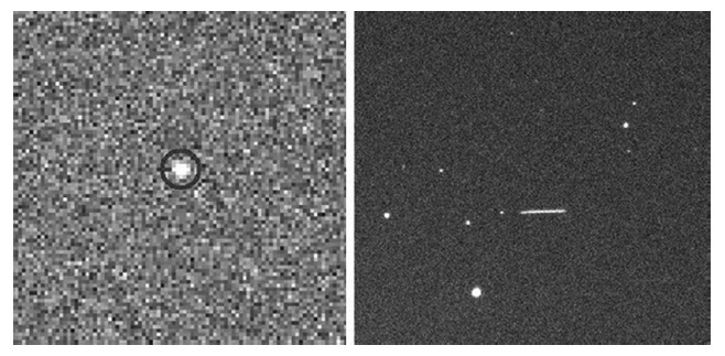
Optical observation data of a satellite can be obtained through the analysis of image from the charge coupled device (CCD). In the star tracking mode of a telescope, stars are shown as points whereas satellites are shown as streaks. On the contrary, only the target satellite is found as a point in the satellite tracking mode. The shapes of the streaks and points corresponding to satellites are similar to those of the streaks and points corresponding to stars. The satellite images can be interpreted by applying the point spread function (Lopez Moratalla et al. 2009).

We observed the COMS to compare the satellite im-age positioning and observation strategies. The COMS is located at longitude 128.2 degree. We employed a 0.6 m wide-field telescope in Daedeok observatory on the Lee Wonchul Hall at the Korea Astronomy and Space Science Institute (KASI, latitude: 36.3982 degree, longi-tude: 127.375 degree and altitude: 0.124 km). The tele-scope, which is a wide-field telescope fabricated for the Near Earth Space Survey project, was originally prepared for the observation of near earth objects (NEO) but it is also suitable for satellite observation thanks to the wide field and rapid driving rate. The field of view (FOV) of the telescope with a 2k CCD is about 1 × 1 degree. The ob-servation was performed between May 16 and July 5 in 2011. The actual number of observation days was six. The COMS was intensively observed during the observation period.

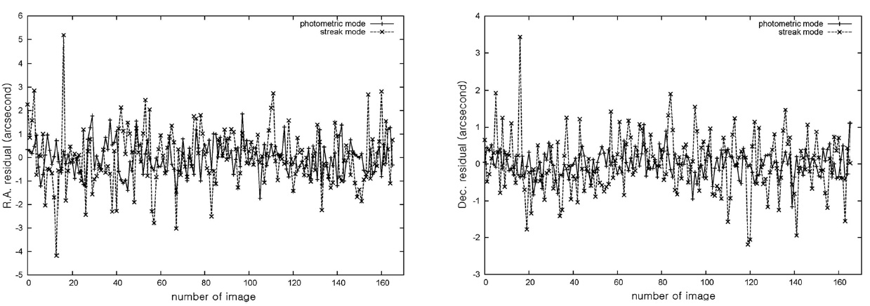
Suitable observation strategies were used for the two image positioning methods. The mount was operated in the general star tracking mode. The first observation strategy was a ‘streak method’ in which the observation was performed with an appropriate level of exposure so that the satellite could be shown as a streak with a suf-ficient number of fixed stars. The second observation strategy was a 'photometric method' in which the obser-vation was performed with a short exposure so that the satellite could be shown as a point like stars. To exclude other factors that could influence the final precision of satellite positioning, we implemented the two strategies one by one. The other factors include atmospheric scat-tering depending on the altitude, positional change of the satellite, weather and the characteristics of the observa-tional instrument. The observation was performed once a minute. However, the respective observation strategies were randomly applied in the period of 2-5 minutes due to the problem of the observation software. Fig. 1 shows the observation results by the photometric method (left) and the streak method (right).

The accuracy of the time when the satellite is observed is important for precise positioning. We synchronized the CCD-controlling computer and the telescope-controlling computer using a time server. The two computers em-ployed Windows and Linux as the operation system, re-spectively. We employed the time server provided by the Korea Research Institute of Standards and Science for the time synchronization.

To verify the precision of the CCD imaging time, we checked it using a camcorder. The observation schedule was prepared using the actual observation software so that the observation schedule can be performed at ev-ery minute for 100 minutes, and the motion of the CCD shutter was shot using a 30-fps camcorder. The exposure time setting was 0.2 sec. The mean error of the CCD shut-ter opening time was 0.073 seconds and the root mean square (RMS) error was 0.039 seconds. The mean time taken for the actual shutter to be opened and for the light to come into the CCD was 0.271 seconds and the RMS error was 0.017 seconds. Thus, the difference should be

corrected by verifying the actual observation start time recorded on the shutter.

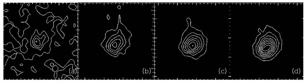
The test observation was performed to obtain the ex-posure time appropriate to the photometric method, the second observation strategy. The mean seeing of the Daedeok Observatory is 3 arcseconds. The angular veloc-ity of the geostationary satellite is about 15 arcsec/sec. Thus, the observation time within 0.2 seconds is secured theoretically. Considering the maximum speed of the used CCD shutter, the test observation was performed at every 0.1 seconds. Fig. 2 shows the contour map of the observed images. It can be found that the image started to be spread to the side after 0.3 seconds. Thus, the ex-posure time appropriate to the photometric method at the current observation system was determined to be 0.2 seconds.

The processing of the observed images was in the fol-lowing orders: firstly, the bias and dark images were cor-rected in the observed images. Then, the world coordina-tion system (WCS) solution was acquired to correct the pointing error of the satellite. General Star Catalogue 1.2 (GSC 1.2) was used for the WCS. Next, the distortion of the satellite images was corrected. We employed the U.S. Na-val Observatory Catalogue (USNO-B1.0) for the distortion correction. There was almost no image distortion since the FOV of the images was less than 1 degree. The error in the processed images was just the error of the used cata-logue, which was less than 1 arcseonds.

The satellite positioning by the streak method, the first observation strategy, was as follows: The starting point of the satellite, shown as a streak in the image, was checked out by the observer's eye. The thickness of the streak was 4 pixels, and the end region showed brightness variation about 2 pixels. Thus, the satellite position should be de-termined within 8 square pixels. The endpoint was deter-

mined assuming the position that was most likely to be the endpoint as the satellite position. Subjective standard might have been involved in this method and the deter-mination was difficult if the image was blurred by the weather.

The satellite positioning by the photometric method, the second observation strategy, was as follows: different from the streak method, the satellite and the stars could not be distinguished in the photometric method. Thus, the position of the satellite was verified on the basis of the position calculated with the orbit information. Since there is almost no change in the altitude and azimuth of a geostationary satellite, the satellite can be identified by comparing the observed images over time. The satellite position was determined on the basis of the identified satellite images and the image reduction and analysis fa-cility. Stars were identified in the observed images, and the satellite position was determined through aperture photometry. The satellite position was determined by the software as the center of a point of satellite shape.

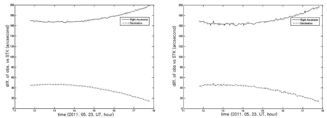
The simulation result was used to compare the sat-ellite observation result. The observation results were compared using satellite toolkit (STK) and two line ele-ments (TLE). The used orbit propagator was Simplified General Perturbations Model 4 (SGP4). The TLE we used was published on May 20. According to Kelso (2007), TLE may show errors of few or dozen of Kilometers in some cases. Fig. 3 compares the observation result and the sim-ulation result. The left compares the result by the photo-metric method and the right compares that by the linear method. The maximum error in the Right Ascension was 200 arcseconds and that of the Declination was 40 arcsec-onds. The observation precision was within the TLE error range.

To compare the positioning precision, we compared the RMS errors in the Right Ascension and Declination of the two observation methods. Fig. 4 shows the com-parative result. After fitting the observation data to the cubic equation over time, the RMS error for the differ-ence was calculated. In the photometric method, the RMS error of the Right Ascension was 0.686 arcseconds and that of the Declination was 0.345 arcseconds. In the streak method, the RMS error of the Right Ascension was 1.242 arcseconds and that of the Declination was 0.810 arcseconds. The RMS error of the streak method is about two times greater than that of the photometric method. The difference in the RMS error of the Declination was greater, which was because the range of determination in the Declination direction was as large as 4 pixels in the streak method. The satellite position was determined in a smaller region in the photometric method than in the

streak method, but the former was more affected by at-mospheric scattering.

The photometric method and the streak method may be applied in different cases depending on the pros and cons. The COMS is bright enough to be observed within a short exposure time. Additionally, the motion in the Dec-lination direction does not need to be considered since the orbit inclination angle of the COMS is very small. However, the photometric method is hardly applied in the cases where the satellite is faint, the velocity in the Declination direction by the orbit inclination angle is greater than that in the Right Ascension, or a sufficient number of stars are not observed by the effect of the weather. Hence, the photometric method can be mainly applied to geostationary satellites. The streak method is applicable to satellites of all orbits and advantageous to the image position correction because sufficiently many stars can be obtained in the background. However, if the exposure time is long, satellite detection may be failed because of the background noise. As regards the streak method, a study was conducted on the precise position-ing by the respective application of appropriate functions to the cross section and length of the streak (Lopez Mo-ratalla et al. 2009).

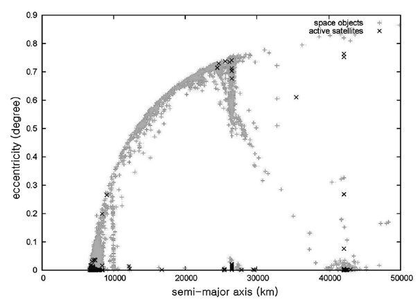
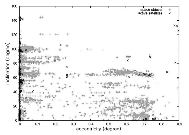
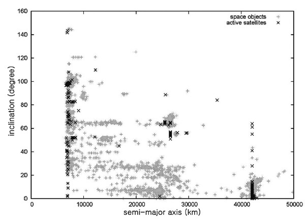
The characteristics of space objects were categorized according to the orbit information. As described before, the number of space objects under tracking is about 15,000. About 1,100 of the tracked space objects are ac-tive satellites (Celestrak 2011). Individual space objects come to have different orbit element characteristics according to the purposes of launchs. Thus, we categorized space objects according to the orbit element character-istics. The used orbit information of space objects is for the orbit calculation in STK and includes the orbit infor-mation of about 15,000 space objects with the satellites in operation distinguished. Fig. 5 shows the semi-major axis and eccentricity of the space objects. The eccentricity of the active satellites is very small, but other space ob-jects have a wide range of eccentricity. The eccentricity of other space objects is increased as the semi-major axis is increased since the space objects with a small semi-major axis and a large eccentricity are dissipated when they enter into the atmosphere. The space objects with the semi-major axis of about 26,000 km and various ec-centricities seem to be the geosynchronous transfer orbit (GTO) space objects. Fig. 6 shows the semi-major axis and orbit inclination angle of space objects. Low earth orbit satellites have various orbit inclination angles. Medium earth orbit satellites are the GPS satellites whose inclina-tion angle is about 50 degree and they seem to be in oper-ation. The orbit inclination angle of the high altitude orbit satellites in operation is between 0 and 20 degree. This in-dicates that the orbit inclination angle is dependent upon the operation purposes of the satellites. Fig. 7 shows the eccentricity and orbit inclination angles of space objects. The eccentricity of the space objects in operation is very small. The space objects having a great eccentricity may be considered on the Molniya orbit or the GTO orbit.

There are seven geostationary satellites that have been operated by Korea, and five of them are currently in op-eration as of April 2011. Most of them stay on the geosta-tionary orbit with an extremely small inclination angle. All the geostationary satellites in operation can be observed in Korea. The surveillance of the Korea geostationary sat-ellites is performed by monitoring the five zones with the optical observation facilities in Korea. If the observation is performed in this manner, a satellite with a great in-clination angle stays within the observation zones for a very short period of time. Additionally, the space objects that may be a potential threat for having the eccentricity and mean movement angle different from those of geo-stationary satellites also stay in the observation zone for a short moment and then disappear. A geosynchronous satellite of a foreign country has already threatened the COMS satellite, and unidentified space objects can be a risk factor always. IOD with a sufficient level of precision as well as an efficient observation strategy is required for the follow-up observation.

The methods to determine the initial orbit using the angle-only information can be categorized by the num-ber of required observation data. The position and veloc-ity of a space object consist of six pieces of information, and thus at least six or three set of 2-type angle-only infor-mation should be acquired. The methods to acquire the three observation data include Gauss, Laplace, r-iteration and Gooding method. The first three methods, which have been known since a long time before, are applied in the research of satellites as well as NEO. Various studies were conducted on the precision of the methods depend-ing on the observation time span and the orbit of the tar-get. The Gooding method, which determines the orbit of a satellite through iteration based on assumed initial val-ues, is known to have a higher level of precision than that of other methods (Escobal 1976, Gooding 1994, Fadrique et al. 2011). Some IOD methods require only two obser-vation data. These include Vaisala and null eccentricity methods. The Vaisala method, which is usually applied to the orbit determination of asteroids, sets an observed position as a perihelion or a perigee. The null eccentric-ity method assumes the eccentricity to be zero and the anomaly to be an arbitrary value (Piergentili 2006). The purpose of this study is the follow-up observation of the unidentified space objects that have been verified during the geostationary satellite observation. Therefore, IOD should be carried out efficiently with a small number of observation data. For this, we employed the null eccen-tricity method.

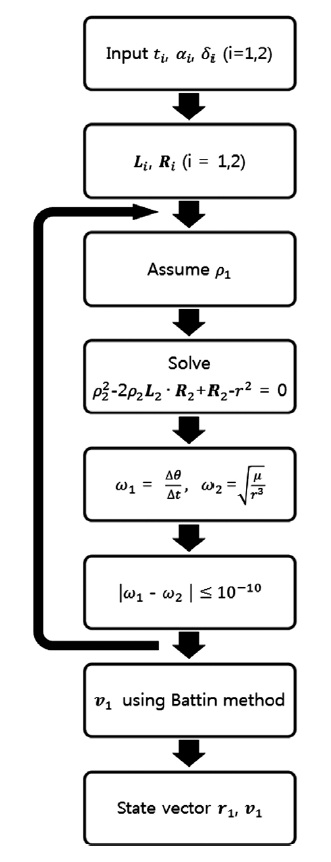
The null eccentricity method is applicable to the space objects having a circular orbit. Since the eccentricity is assumed to be zero, no perigee can be designated. Fig. 8 shows the process of the null eccentricity method. Two observation data are used for one arc. One or two ob-servatories are used but the observation time should be different with each other. Assuming the range between the target space object and the observatory to be ρ₁, the range from the Earth's center to the space object, r, can be determined. Since the eccentricity is assumed to be zero, the distance, r, is equal at each observation time. Through this, the range between the target space object and the observatory at the second observation time, ρ₂, can be de-termined. The angular velocity of the satellite, ω₁, can be calculated with the observation time span and the angle between the two satellites. The angular velocity by gravity,

ω₂, can be also calculated with the distance determined earlier, r. Since two-body motion is considered, the two calculated angular velocity values should be equal. Cor-rection of ρ₁ is performed by comparing the difference be-tween the two angular velocity values. After the actual r is determined by repeating this process, the velocity of the space object at the initial observation time is calculated by the Battin method (Vallado & McClain 2001). The po-sition and velocity of the satellite at the first observation time are finally obtained.

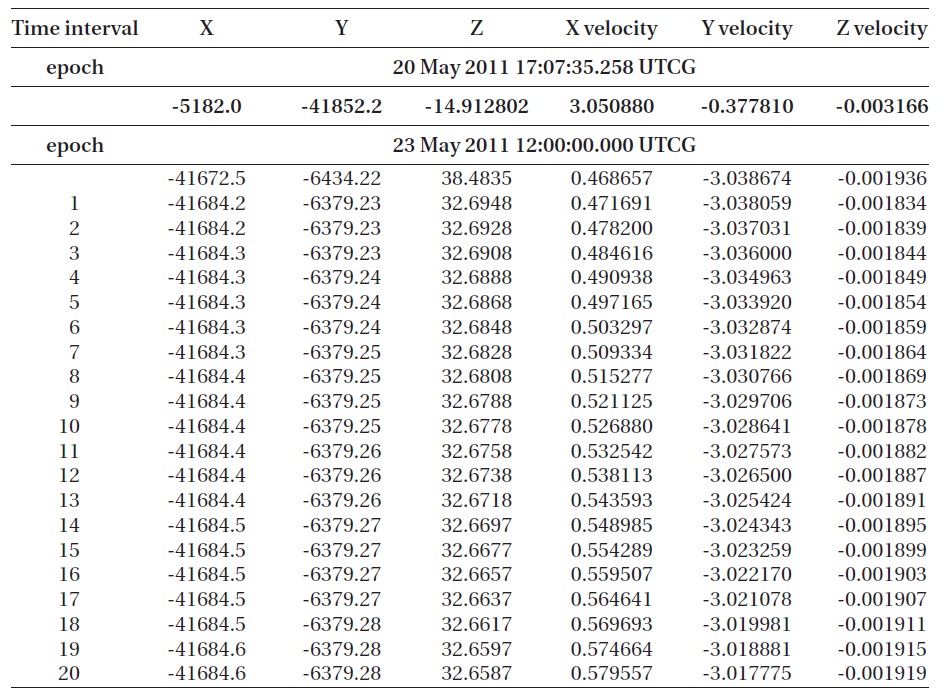
We performed an experiment by applying the null ec-centricity method to the simulation data. The subject of simulation was the COMS, and the simulation was per-formed using the TLE information and the orbit propa-gation by STK. The used orbit propagator was SGP4. Only one TLE was used to eliminate the effect of orbit change by the station keeping maneuver. The propagated ephemeris was used as the true value. The performance of the null eccentricity method was verified by increas-ing the observation time interval from 1 to 20 minutes. The ground station was set to be the Lee Wonchul Hall in KASI. Table 1 shows the epoch and state vector in the

orbit propagation and the epoch and state vector after the orbit determination. The orbit determination results are also shown along with the time span. The epoch of the or-bit elements used in the orbit propagation was different from the epoch at the time when the orbit determination was actually performed because the orbit elements used in the orbit propagation were converted from the actually published TLE and the actual orbit determination time was set to be similar to the actual observation time. After the experiment, the actual observation data were used for the orbit determination. For the orbit determination, we generated the Right Ascension and Declination observa-tion data using J2000 in one minute interval. The result of the orbit determination had an error of about 50 Kilo-meter with the initial value. This error was applied almost identically to all the time intervals. However, when the orbit propagation was begun, the error was gradually in-creased and then decreased to be the minimum after one period, and the entire variation was repeated.

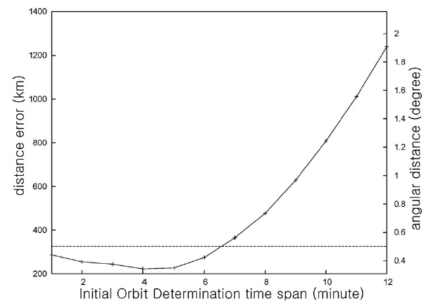
For the next, the IOD result was propagated and the results were compared. The orbit propagation period was 10 days. Since the null eccentricity method considers only two-body motion, the orbit propagation should also consid-er only two-body motion. However, we de-cided to use SGP4 as the orbit propagator in order to verify what result is actually brought about by the orbit determination result in the situation where there are vari-ous perturbations. The error of the IOD was expressed in the unit of distance because it is convenient in analyzing the characteristics of the orbit determination method when compared with the Right Ascension and Declina-tion projected on a two-dimensional plane. The distance error can be considered as the maximum error range of the angular distance to the space object predicted on the celestial sphere. The distance on the celestial sphere was converted into an angle and shown on the right side of the plot below with the dotted line representing the angle of 0.5 degree that is corresponding to the half of the view-ing angle. Fig. 9 shows the RMS errors in the orbit propa-gation performed for 10 days in one hour interval. The result indicated that the RMS error was increased as the

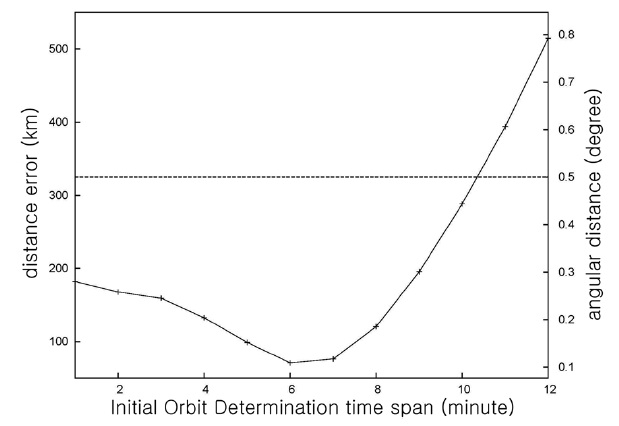
time span was increased. Except the time span under 6 minutes, the RMS error was greater than 0.5 degree at all the time spans. Fig. 10 shows the RMS errors calculated with respect to the time of the orbit determination after the orbit propagation of 10 days. Since the precision of the time used for the orbit determination was much high-er than that of other times, the actual difference was com-pared. The dotted line here also represents the angle of 0.5 degree converted into the distance on the geostation-ary orbit. The RMS error for the ten days was smaller than 0.5 degree for the time spans of 10 minutes or less. The local minimum was found when the time interval was 6 minutes. As shown in Fig. 5, most of the space objects around the geostationary orbit have the eccentric smaller

than 0.1 and they can be considered to have a circular or-bit. Thus, the method is applicable to most of the space object that may threaten the geostationary satellites of Korea. In addition, the method showed a better result with the limited observation data with an extremely short observation span than that of the general IOD method. The result was more accurate than even that of the meth-ods to calculate six orbit elements using three observa-tion data (Musci et al. 2004, Porfilio et al. 2006). The result of the null eccentricity method was more excellent than that of the Lambert method or the Laplace method for a Low Earth Orbit satellite (Piergentili et al. 2005).

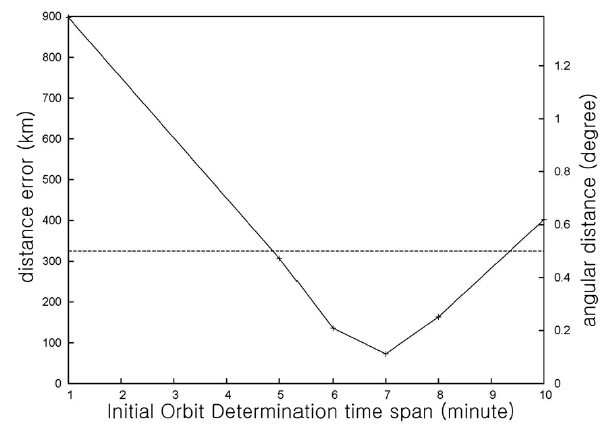
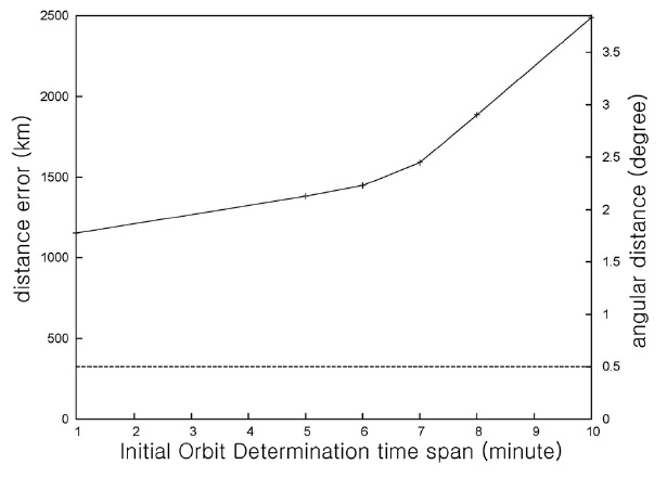
Next, we determined the initial orbit using the actual observation data. The used observation data were the COMS observation data on May 23, 2011. The satellite positioning method was the photometric method. As mentioned before, the orbit calculation could not be per-formed in one minute unit as in the case of the simulation because the observation interval was not uniform. The time intervals were 1, 5, 6, 7, 8 and 10 minutes. Since the RMS error was 0.5 or greater when the time interval was 10 minutes or longer in the previous simulation result, we used only the observation data with the time interval of 10 minutes or less. Fig. 11 shows the RMS error calcu-lated by performing the orbit propagation for 10 days in one hour interval with the IOD result based on the actual observation data. The difference with the simulation re-sult was great when the time interval was short. The error was with 0.5 degree continuously for the 10 days at none of the time intervals. Fig. 12 shows the RMS error based on the time used for the orbit determination calculated after performing the orbit propagation for 10 days with the IOD result based on the actual observation data. The

error was less than 0.5 degree at all the time spans except one and ten minutes. The effect of the observation error was greater than that of the time span.

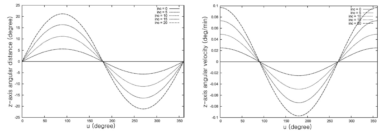
In general, the motion of space objects in the Decli-nation direction is determined by the orbit inclination angle. As shown above, most of the high altitude objects have the eccentricity close to zero and the orbit inclina-tion angle of 20 degree or less. Thus, most unidentified space objects approaching geostationary satellites have similar orbit characteristics. To establish the observation strategy for effective IOD of unidentified space objects, not only the observation interval but also angular velocity of the target space object should be taken into account.

In case of a circular orbit with an orbit inclination an-gle, the z-axis movement and velocity can be calculated by the following equation (Vallado & McClain 2001):

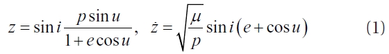
where i denotes the orbit inclination angle, p the semi-latus rectum and e the eccentricity. Since there is no peri-gee when a circular orbit is assumed, there is no anomaly. Hence, the argument of latitude, u, calculated by adding ω and υ is used. Fig. 13 shows the z-axis distance and ve-locity of the geosynchronous satellite viewed from the Daedeok Observatory calculated with respect to the ar-gument of latitude for the respective orbit inclination angles. The inclined geosynchronous satellite penetrates the equator two times a day at the ascending node and the descending node. The angular velocity on the right side shows that the angular velocity of the satellite was the maximum at the moment when it was penetrating the equator. This suggests that space objects are at their maximum angular velocity when passing around the geo-stationary satellite. The velocity at the ascending and de-scending nodes is depending on the orbit inclination; the angular velocity is greater if the orbit inclination is great-er. It takes about five minutes for a space object with the orbit inclination of 20 degree to pass through 0.5 degree, while it takes 25 about minutes for a space object with the orbit inclination of 5 degree to pass through 0.5 degree. When determining the observation period, the angular velocity of the satellite should be taken into account. If the time span appropriate for the IOD is assumed to be 1-10 minutes, the observation needs to be performed two times within five minutes in order to observe the satellite with the orbit inclination up to 20 degree for more than two times.

An effective observation strategy is required to perform the IOD for the follow-up observation of unidentified space objects. When a geostationary satellite is in surveil-lance, the observation time is affected only by the relative angle between the Earth’s shadow and the solar position. Thus, the foremost criterion for the observation period is to maintain the orbit determination precision for the surveillance target satellite. Next, if an unidentified space object is observed, the IOD needs to be carried out for the follow-up observation. In the case where the null eccen-tricity method is applied, if the observation is performed two times within 10 minutes using a telescope of which viewing angle is 1 degree, the follow-up observation can be performed at either the next ascending node or the next descending node. However, in case of a space object with the orbit inclination of 20 degree or less, it takes at least five minutes to get out of the viewing angle from as- cending node or the descending node. Hence, if the geo-stationary satellite observation is performed so that it can be observed two times within 1-5 minutes, the follow-up observation of a space object with the orbit inclination of 20 degree or less can be successfully performed through the IOD.

The geostationary satellite surveillance mission in-cludes prediction of collision with other space objects. The precision of the observation data should be increased for the orbit determination of space objects. We tested two observation and positioning methods, the streak method and the photometric method, in order to elevate the satellite image positioning precision for space objects. The photometric positioning method is more ac-curate than streak method for geostationary satellites, but the weather, brightness of the target satellite and the inclination should be taken into account.

We also tested the null eccentricity method as a meth-od to determine the initial orbit for the follow-up obser-vation of unidentified space objects. The null eccentricity method is suitable for the IOD of the space objects found by the geostationary satellite surveillance. The simulation result showed that the time interval needed for effective IOD was 1-10 minutes which is shorter than that of other methods. This means that the orbit inclination constraint is relatively great with respect to the unidentified space objects whose initial orbit can be determined.

In the geostationary satellite surveillance, the follow-ing observation strategy should be considered to deter-mine the initial orbit of the observed unidentified space objects by the null eccentricity method and perform the follow-up observation based on the IOD result: first, the observation for same area should be performed two times within 10 minutes, considering the precision of null eccentricity method as the IOD method. Next, assuming that the unidentified space object is on an inclined geo-synchronous orbit, the observation should be performed two times within five minutes if the orbit inclination is 20 degree or less. Hence, if the observation is performed two times within five minutes in the geostationary satellite surveillance strategy, the follow-up observation is able to be performed with the unidentified space objects which have inclined geosynchronous orbit with inclination un-der 20 degree found during the observation.

Following additional studies need to be conducted for the tracking of unidentified space objects that may col-lide with geostationary satellites. The unidentified space objects having the possibility of collision with geosta-tionary satellites include not only the geosynchronous space objects but also the GTO space objects having a great eccentricity. The apogees of the latter ones are close to the geostationary orbit, and they pass through differ-ent position at each time. Other IOD methods should be considered, not the null eccentricity method, for the GTO space objects. These objects are hardly observed by the photometric method. Therefore, the endpoint determi-nation precision should be increased in the streak meth-od. Many studies have been conducted on the endpoint determination precision in the linear observation meth-od. A comparative study of the IOD methods needs to be performed with respect to various orbits on the basis of the research results. By means of this, an effective surveil-lance may be able to be performed with the space objects on the geostationary orbit.