In this paper, the authors introduced a new approach to find the optimal collision avoidance maneuver considering multi threatening objects within short period, while satisfying constraints on the fuel limit and the acceptable collision probability. A preliminary effort in applying a genetic algorithm (GA) to those kinds of problems has also been demon-strated through a simulation study with a simple case problem and various fitness functions. And then, GA is applied to the complex case problem including multi-threatening objects. Two distinct collision avoidance maneuvers are dealt with: the first is in-track direction of collision avoidance maneuver. The second considers radial, in-track, cross-track direction maneuver. The results show that the first case violates the collision probability threshold, while the second case does not violate the threshold with satisfaction of all conditions. Various factors for analyzing and planning the optimal collision avoidance maneuver are also presented.
Space debris or space junk refers to the uncontrollable objects among the artificial objects in the space. At pres-ent, it is estimated that there are about 22,000 pieces of space debris larger than 10 cm and more than 600,000 pieces larger than 1 cm with over millions of tiny space debris smaller than 1 cm (Liemer & Chyba 2010).
The number of space debris has been greatly increased in recent times especially by the interception experiment of the Chinese FengYun 1C in January, 2007 and the colli-sion of the IRIDIUM 33 of the USA and the COSMOS 2251 of Russia in February, 2009. Thus, there is an increasing interest in the number of space debris worldwide. The USA, the space development frontier, and the European Space Agency (ESA) have already developed the system for the analysis of space debris collision risk and utilized it for the satellites of their countries (Morris 2004, Mariel-la 2006). However, the space debris collision risk analysis systems that have been developed until now do not pro-vide any specific maneuver information for avoidance, just analyzing the risk of collision.
With regards the avoidance maneuver, ESA has con-ducted active studies on the collision avoidance meth-ods based on variation of the orbit period or semi major axis, the timing of collision avoidance maneuver, and the change of the collision probability by the thrust direction at the expected collision timing (Alfano 2005, Sanchez-Ortiz et al. 2006). The collision avoidance method to in-crease the semi major axis and orbit period through the in-track direction velocity increment is often chosen in general because it consumes less fuel, according to the result. However, in the studies, the number of approach-ing space debris was assumed to be one, the position of the performing the collision avoidance maneuver was limited to the expected position of collision or the posi-tion half period before the expected position of collision, or the thrust direction of the collision avoidance maneu-ver was limited to one axis or two axes direction of the radial, in-track, cross-track (RIC) coordinates.
In our study, we investigated the optimized collision avoidance maneuver method, considering the issues that have not be taken into account, i.e. the multiple ap-proaching space debris pieces, the timing of collision avoidance maneuver and the velocity increment to the three directions of the RIC coordinates.
In this study, neither a differentiable object function may be constituted nor may an analytical method be ap-plied, because different analytical methods such as orbit analysis as well as collision probability calculation based on the orbit analytical results. Thus, we employed the ge-netic algorithm (GA) that is relatively robust to this type of problem and useful to obtaining a global solution. The objective function of the GA (fitness function) was consti-tuted for the collision probability and the miss distance.
2. PROBLEM DEFINITION AND ACCESS
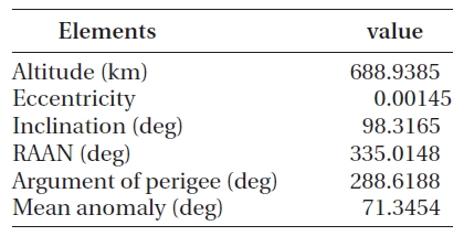
The object chosen for the collision avoidance maneu-ver was the Korea Multi-Purpose Satellite-2 (KOMPSAT-2). The orbit information of the satellite is shown in Table 1.
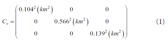
The assumed case was where multiple space debris pieces are approaching the KOMPSAT-2 within a few days. The problem was applied, dividing the case to a simple case and a complex case. The simple case was applied in order to verify the applicability of the optimal solution obtained by the GA by simplifying the collision avoidance maneuver. For the complex case, the space debris orbits were designed so that multiple space objects may be ap-proaching in order to compare the conventional collision avoidance maneuver methods and the one suggested in this study. The size of all the approaching space debris pieces was assumed to be 10 cm. The covariance matrix
[Table 1.] Orbit information of KOMPSAT-2.

Orbit information of KOMPSAT-2.
of the individual pieces was assumed as shown in Eq. (1):
2.1 Calculation of the Collision Probability
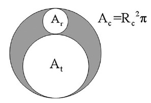
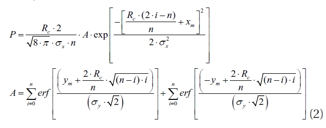
On the B-plane with the satellite at the center, the space debris approaches perpendicularly. Connection of the same values of the collision probability calculated with the positions of the satellite and the space debris as well as the positional uncertainties gives the elliptical shape shown in Fig. 1.
AdvCAT® of STK using the Alfano formula was em-ployed for the calculation of the collision probability. Eq. (2) shows the Alfano formula used in AdvCAT® (Alfano 2007):
where
The GA applied to this study is known to have excellent convergence to global minimum or maximum in various application problems compared with other optimization algorithms (Goldberg 1989).
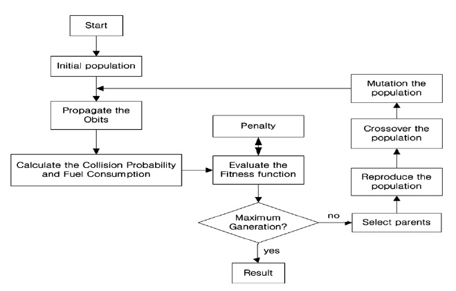
The optimization processes based on the GA realized in this study were the Matlabⓡ GA and the AGI STK/Adv-CATⓡ software for the prediction of the orbit and the cal-culation of the collision probability (Kim et al. 2009). Fig. 3 shows the algorithm flow chart of the realized process.
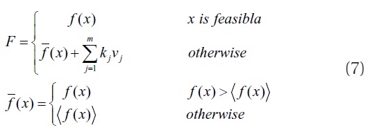
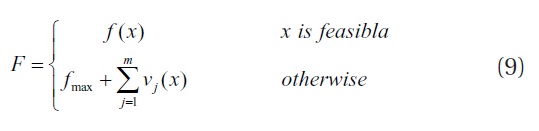
As shown in Fig. 3, the initial group generated by the GA was applied to assess the probability of collision with multiple pieces of space debris. Then, the objective func-tion (fitness function) was acquired by reflecting the amount of fuel consumed by the orbit maneuver through penalizing strategy. The most widely used fitness function has the form described in the article ‘Algorithms and Ex-amples’ by Deb & Agrawal (1999) as shown in Eq. (3):
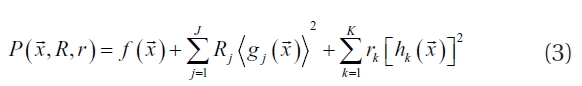
where

denotes the objective value to be minimized and
and
the constraints.
After the selection, crossover and mutation of the GA are performed, the newly generated variables are applied to calculate the objective function once again. The pro-cess of the GA was to be ended when the maximum num-ber of generation is reached.
The most important thing in this process is the fitness function that is directly involved in the regeneration of the objects. The optimum solution can be obtained more rapidly and precisely depending on the fitness function
values. In this article, three fitness functions are intro-duced and the results are compared.
3. SIMULATION RESULTS AND SUMMARY
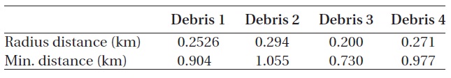
If the problem case is simplified, the optimum solution that satisfies the constraints is predictable. The study for the simple case was performed to verify the applicability of the optimization method by comparing the GA opti-mal solution with the predicted optimal solution. Table 2 shows the space debris of which elevation is different from that of the KOMPSAT-2 but close to it.
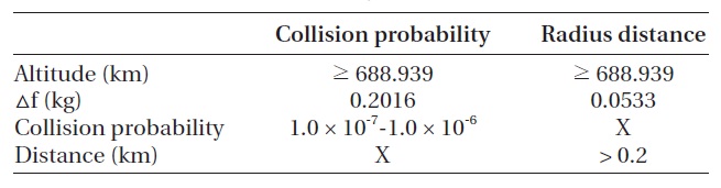
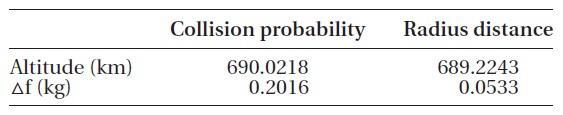
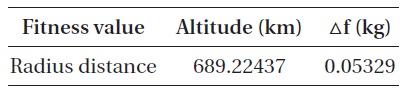
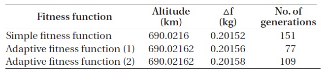
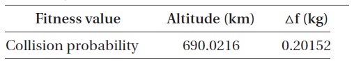
In this study, the collision probability and the distance in the radius direction were analyzed as the objective values. The collision probability of 1.0 × 10⁻⁷~1.0 × 10⁻⁶ or the miss distance of 0.2 km or more is expected for all the pieces of the space debris. Table 2 shows the predicted transfer orbit following the collision avoidance through elevation increase. To satisfy the allowable collision prob-ability, the orbit will be transferred to 690.0218 km as the elevation is increased by 1.0833 km after consuming 0.2016 kg of the fuel. To satisfy the allowable radius dis-tance, the orbit will be transferred to 689.224 km as the el-evation is increased by 0.285 km after consuming 0.0533 kg of the fuel. Fig. 4 briefly expresses the orbit shape of the KOMPSAT-2 and the space debris pieces and the orbit transfer by the maneuver.
[Table 2.] Information of space debris at simple case.

Information of space debris at simple case.
Each objective value has different constraints for op-timization. Table 3 shows the individual constraints. The constraint that the elevation should be higher than 688.939 km is because the elevation of the optimal solu-tion is predicted to be higher than that current elevation (688.939 km). Low earth orbits basically adopt the strat-egy to increase the elevation for the collision avoidance maneuver because they have natural elevation decrease. With regard to the fuel condition, the constraint of the fuel consumption of the predictable optimum solution
[Table 3.] Constraint according to objective.

Constraint according to objective.
[Table 4.] Setting of genetic algorithm for simple case.

Setting of genetic algorithm for simple case.
[Table 5.] Result of genetic algorithm (objective is acceptable collision probability).
Result of genetic algorithm (objective is acceptable collision probability).
[Table 6.] Estimated result according to objective.

Estimated result according to objective.
[Table 7.] Collision probability and range (objective is acceptable collision probability).

Collision probability and range (objective is acceptable collision probability).
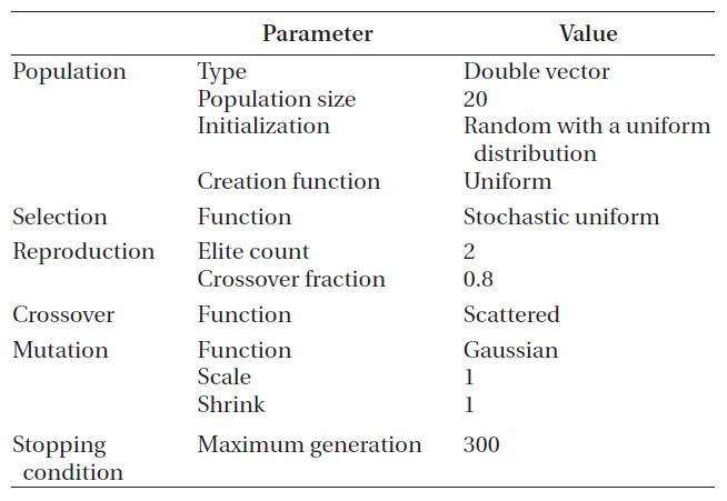
is adopted so that the consumption may not exceed the value. The allowable probability of collision with the indi-vidual pieces of the space debris is 1.0 × 10⁻⁷~1.0 × 10⁻⁶ and the allowable radius distance is 0.2 km or higher. Table 4 shows the settings of the GA applied to obtain the opti-mum solution for the simple case.
3.1.1 Simulation Result--Collision Probability
The fitness function described in Section 2.2 was con-stituted for the collision probability as shown in Eq. (4):
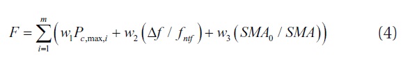
where
Penalty is given including the weights w1, w2 and w 3 each time when the constraints in Table 3 are violated. The
The fitness function of Eq. (4) was applied to the GA, and the result showed that all the constraints in Table 3 were satisfied, as shown in Table 5.
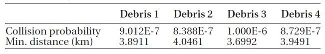
The optimum solution of the GA was found to be very close to the results predicted in Table 6. Table 7 shows the probability of collision and miss distance with the pieces of the space debris after the collision avoidance maneuver.
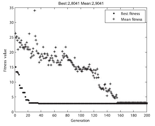
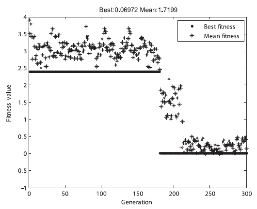
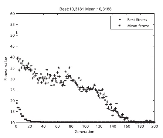
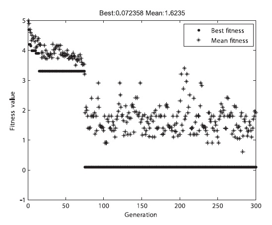
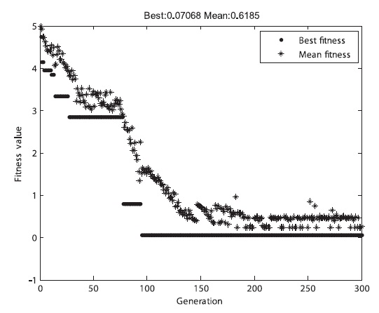
As shown in Table 7, the allowable collision probability was satisfied for all the pieces of the space debris. Fig. 5 shows the GA result of the fitness function. The specific shape of the graphs was different at each time of the sim-ulation, but all of them converged and calculated opti-mum solutions were similar.
3.1.2 Simulation Result--Miss Distance
The fitness function mentioned in Section 2.2 was con-stituted for the collision probability as shown in Eq. (5):
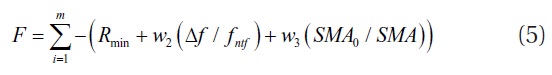
where
Penalty is given including the weights
The fitness function of Eq. (5) was applied to the GA, and the result showed that all the constraints in Table 3 were satisfied, as shown in Table 8.
The optimum solution of the GA was found to be very close to the results predicted in Table 6. Table 9 shows the probability of collision and miss distance with the pieces of the space debris after the collision avoidance maneuver.
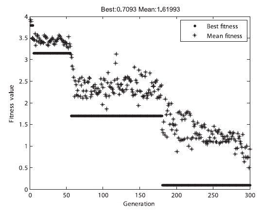
As shown in Table 9, the allowable miss distance was satisfied for all the pieces of the space debris, which is the same result of the predicted optimum solution. Fig. 6 shows the GA result graph. The specific shape of the graphs was different at each time of the simulation, but all of them converged and calculated optimum solutions were similar.
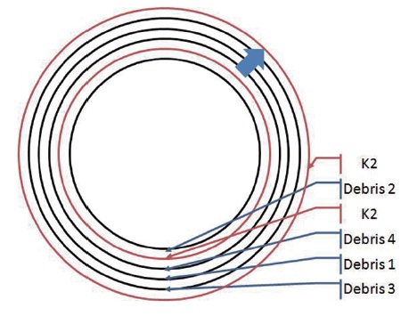
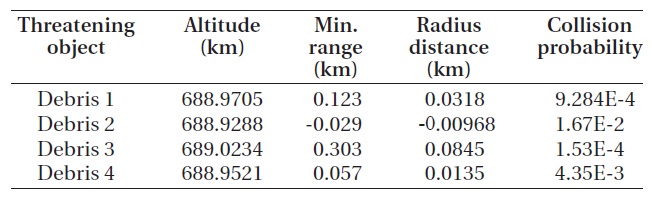
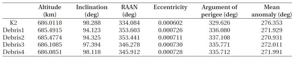
To constitute a complex case, the orbit was set for mul-tiple pieces of the space debris to approach the satellite. The pieces of the space debris were generated as shown in Table 10 by altering all the orbit elements of the KOMP-SAT-2. Table 11 shows the collision probability and the miss distance between the individual pieces of the space debris and the KOMPSAT-2. The avoidance maneuver method considered not just one in-track direction but all the three directions of radial, in-track and cross-track in order to compare the result with that of the conventional studies.
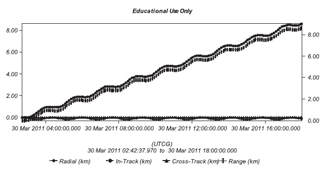
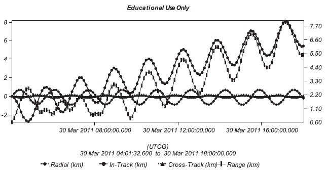
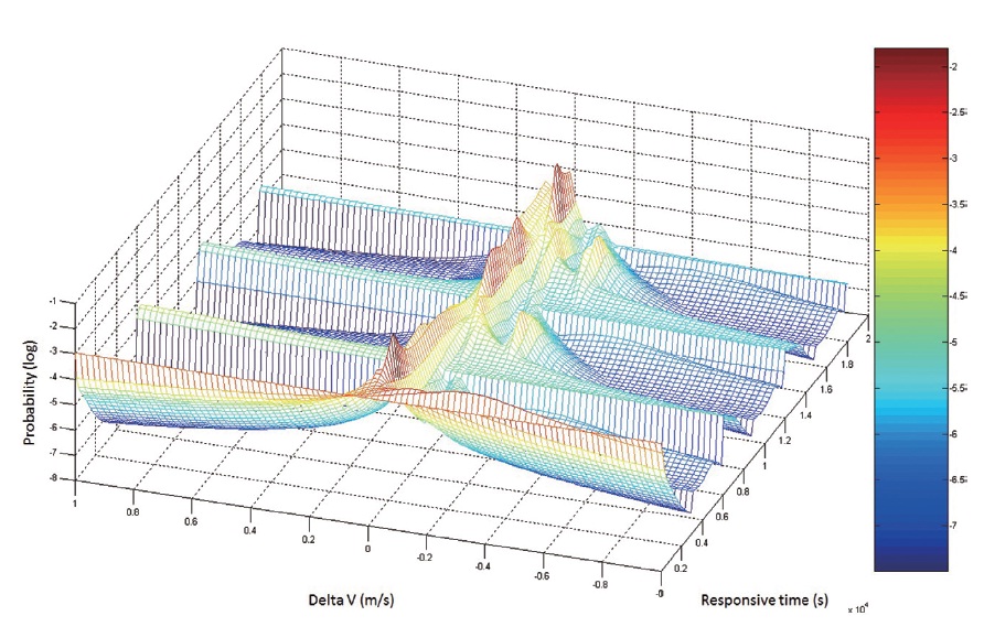
Fig. 7 shows the change of the collision avoidance ma-neuver timing and the collision probability between the Debris 4 in Table 10 and the KOMPSAT-2 by the velocity increment. The direction of the velocity increment was limited to the in-track direction. Fig. 7 shows that the col-lision probability was greatly influenced by the collision avoidance maneuver timing and the velocity increment. The collision avoidance maneuver timing is closely relat-ed to the satellite operation relevant to the mission, and it changes the collision probability by greatly affecting the
[Table 8.] Result of genetic algorithm (objective is acceptable radial distance).

Result of genetic algorithm (objective is acceptable radial distance).
[Table 9.] Radial range and range (objective is acceptable radial distance).

Radial range and range (objective is acceptable radial distance).
relative distance and period. The collision direction and the velocity increment have a direct effect on the transfer orbit. For these reasons, the collision avoidance maneu-ver timing and the velocity increment were set as the in-put variables.
The collision avoidance maneuver timing is decided at the time as close as possible to the time when the colli-sion is predicted, and it is usually 1 or 2 orbits before the predicted collision timing (Alfano 2005). In this study, the time range of the collision avoidance maneuver was set as the time 9,600 seconds before the time when the first collision is expected to occur among the four pieces of the space debris. 9,600 seconds, corresponding to about 2.67
[Table 10.] Orbit information of K2 and debris at complex case.

Orbit information of K2 and debris at complex case.
[Table 11.] Collision probability and RIC, range.
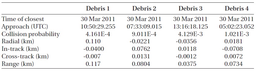
Collision probability and RIC, range.
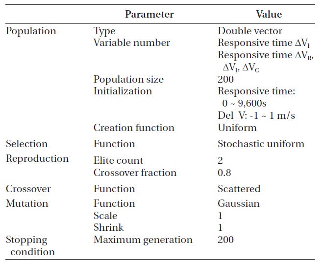
hours, allow about 1.5 orbits until the time when the first collision is expected to occur. Additionally, the in-track direction veloc-ity increment and the RIC direction velocity increment were set as the input variables for the col-lision avoidance maneuver direction in the simulation in order to compare the result with that of the conventional studies. The variable range of the velocity increment in each direction was set to be ±1 m/s. The allowable col-lision probability was set to be 9.9 × 10⁻⁶~1.0 × 10⁻⁶ as the criterion for the optimum collision avoidance maneuver so that it could be satisfied for the four pieces of the space debris. The maximum fuel consumption was limited to 0.3 kg.
Table 12 shows the applied GA settings to obtain the optimum solution for the complex case. Since the ana-lytical range of the variables was wider than that of the simple case, the number of individuals in each genera-tion was increased to 200.
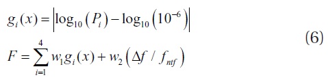
The fitness function introduced in Section 2.2 was applied, and its specific formula is shown in Eq. (6). Al-though minimization of the collision probability was the goal, all the objects are expected to satisfy the allowable collision probability and thus 10-6 was set as the reference value. The fitness function,
The value of
[Table 12.] Setting of genetic algorithm for complex case.

Setting of genetic algorithm for complex case.
[Table 13.] Result of genetic algorithm with in-track maneuver.
Result of genetic algorithm with in-track maneuver.
if the allowable fuel consumption is satisfied; otherwise, 100.
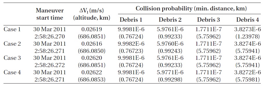
The results of the simulation performed with the input variables of the collision avoidance maneuver timing and the in-track direction velocity increment are shown in Figs. 8 and 9, and Table 13. Table 13 shows the values of
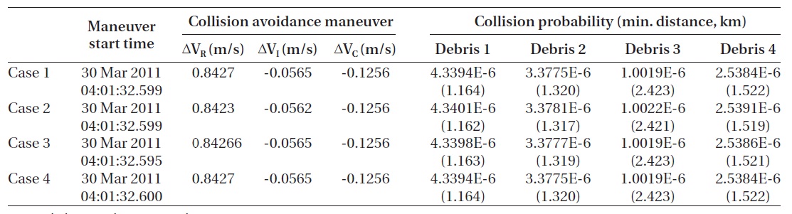
variables of the collision avoidance maneuver timing and the RIC direction velocity increment are shown in Figs. 10 and 11, and Table 14. The result shows that
Comparison of the Table. 13 and 14 indicates that the RIC direction velocity increment requires more than 35 times of increment than that of the in-track direction ve-locity increment. This is because the in-track direction
[Table 14.] Result of genetic algorithm with RIC maneuver.
Result of genetic algorithm with RIC maneuver.
velocity increment does not provide the any case where the given allowable collision probability may be satisfied for the Space Debris 3. The RIC direction velocity incre-ment provides the case where the given allowable colli-sion probability may be satisfied for the Space Debris 3, while satisfying the allowable collision probability for other pieces of the space debris. This can be verified in Figs. 9 and 11 showing the change of the RIC direction distance from that of the time before the collision avoid-ance maneuver. Comparison of the Figs. 9 and 11 indi-cates that the transfer orbit is closer to the previous orbit at the time when the optimum solution appears in the in-track direction velocity increment than in the RIC di-rection velocity increment. Hence, the in-track direction velocity increment dose not satisfy the allowable collision probability for the Space Debris 3, while the RIC direction velocity increment dose.
In other words, when only the in-track direction veloc-ity increment is considered, the allowable collision prob-ability is never satisfied for the Space Debris 3 regardless of the weights. However, when the three RIC directions velocity increment is considered, the allowable collision probability is satisfied. This indicates that, although the in-track direction maneuver is often performed in gen-eral, the maneuver in other directions needs to be con-sidered depending on the case and purpose.
3.3 Analysis of the Fitness Function
In this study, the optimization problem is dealt with us-ing the GA. The fitness function including the objective values and constraints was constituted to solve the maxi-mum or minimum problem. The convergence time and global solution calculation performance of the GA are de-pendent on the fitness functions. In this study, the perfor-mance was compared with regard to the fitness functions.
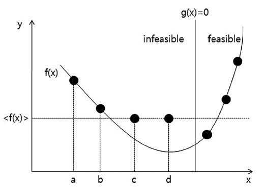
Besides the fitness function described in Section 2.2, there are various fitness functions. The fitness function constituted without setting specific penalty factor values is called adaptive fitness function. In an adaptive fitness function, the penalty factors are determined during the calculation process. Among the various adaptive fitness functions, two methods are introduced in this article. The first one is the method by introduced by Lemonge and Barbosa in 2004 (Helio & Afonso 2008), shown in Fig. 12.
As can be seen from the constitution of the fitness func-tion, the objective function value is selected as the fitness function value in the allowed range, while an alternative value is selected in the constrained range. The greater value between the objective function value (
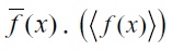
denotes the mean objective func-tion value of the generation that is currently calculated, and
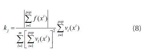
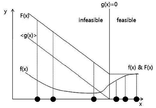
The penalty factor is calculated as the ratio of the sum of the objective function values according to the degree of the violation. The second adaptive fitness function, which is similar to the first one but a little bit simpler, is shown in Fig. 13 (Deb & Agrawal 1999).
As can be seen from the constitution of the fitness func-tion, the objective function value is selected as the fitness function value in the allowed range, while an alternative value is selected in the constrained range.
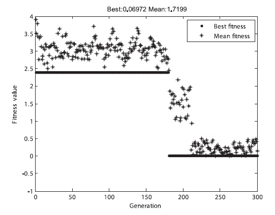
The three fitness functions were applied to the GA for the simple case with respect to the collision probability. The result showed that they satisfied all the constraints in Table 3, indicating that the results were very close to the expected results. The convergence time of the GA was greatly affected by the fitness functions, as shown in Figs. 14-16. Table 15 shows the analytical results of the mean converged generation after 100 times of calculation for each of the fitness functions.
As indicated by Figs. 14-16 and Table 15, the first adap-tive fitness function converged most rapidly, while the basic fitness function converged most slowly. Therefore, an appropriate fitness function should be selected on the basis of the problem case in order to improve the GA per-formance.
The usefulness of the GA was verified by analyzing the optimum collision avoidance maneuver in a simple case and the GA performance depending on the fitness
[Table 15.] Convergence generation according to fitness function.

Convergence generation according to fitness function.
functions, and the optimum solution was calculated by applying it to a complex case. The single in-track direc-tion velocity increment is mostly employed as a collision avoidance maneuver method since it consumes less fuel. However, in the case where performance requirements are given including the allowable collision probability of multiple approaching objects, orbit maneuver timing and minimization of fuel consumption, the maneuver in the three RIC directions has to be taken into account be-cause the collision avoidance maneuver considering only the in-track direction may not satisfy the performance re-quirements. In addition, it is assumed to be important to establish the differentiated optimum collision avoidance maneuver plants considering the characteristics of the individual missions of the current and future KOMPSATs. For example, the collision avoidance maneuver timing may be selected to minimize the mission resting phase as well as the fuel consumption, considering the imaging schedule of a satellite.
In this article, the optimum collision avoidance ma-neuver strategy considering multiple pieces of space de-bris soon approaching was suggested and the validity was verified. The collision probability is greatly affected by the collision avoidance maneuver timing and the velocity increment. The simulation result showed that consider-ation of on the single in-track direction fails to satisfy the allowable collision probability for all the approaching ob-jects whereas consideration of the maneuver in the three RIC directions satisfies the collision probability for all the pieces of the space debris.
Future studies are supposed to deal with more compli-cated problems reflecting the satellite system constraints in the satellite imaging schedule and maneuver.