The world’s first geostationary ocean color imager (GOCI) is a three-mirror anastigmat optical system 140 mm in diameter. Designed for 500 m ground sampling distance, this paper deals with on-orbit modulation transfer function (MTF)measurement and analysis for GOCI. First, the knife-edge and point source methods were applied to the 8th band (865 nm) image measured April 5th, 2011. The target details used are the coastlines of the Korean peninsula and of Japan, and an island 400 meters in diameter. The resulting MTFs are 0.35 and 0.34 for the Korean East Coastline and Japanese West Coastline edge targets, respectively, and 0.38 for the island target. The daily and seasonal MTF variations at the Nyquist frequency were also checked, and the result is 0.32 ± 0.04 on average. From these results, we confirm that the GOCI on-orbit MTF performance satisfies the design requirements of 0.32 for 865 nm wavelength.
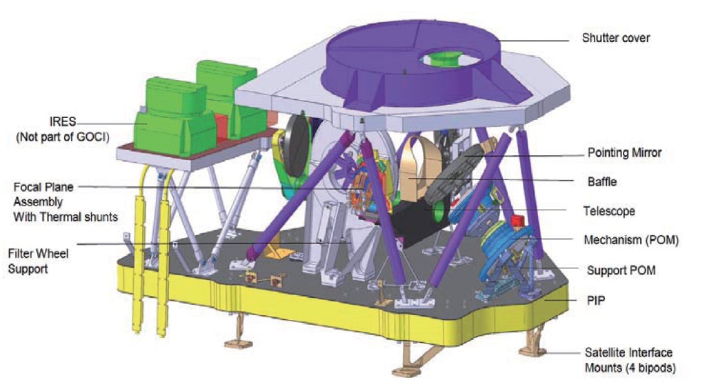
Geostationary ocean color imager (GOCI), launched June 27th, 2010, is the world’s first Geostationary Ocean remote sensing instrument with an effective aperture of 140 mm. The scientific goals of GOCI are 1) monitoring of the ocean environment around the Korean peninsula, 2) observation of oce an ecological system and 3) monitoring of climate change. Fig. 1 shows the GOCI optical system consisting of three mirrors that forms a three-mirror anastigmat (TMA)-type optical system to achieve a compact packaging volume. The GOCI ground sample distance (GSD) indicating spatial resolution is designed to be 500m, which is comparable to that of low earth orbit (i.e. polar-orbit) satellites such as MODIS, MERIS (Xiong et al. 2006).
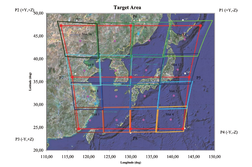
A single observation sequence generates a mosaic of 16 snapshot observation tiles, using a motorized pointing mirror with 2 degrees of freedom as shown in Fig. 2 below. The GOCI image can cover 2,500km at North-South direction and at East-West direction (Cho et al. 2009, 2010). The image data are takenin less than 30 minutes, and it can measure the Korean peninsula 8 times a day for high temporal resolution.
The on-orbit modulation transfer function (MTF) measurement is a popular choice for high-resolution satellite performance analysis. Examples may include, but are not limited to, IKONOS (Cook et al. 2001, Choi 2002), OrbView (Crespi&Vendictis 2009), SPOT (Viallefont&Leger 2010) and KOMPSAT (Hwang et al. 2008). In particular, SPOT used the knife-edge method for its on-orbit MTF measurement and analysis (Viallefont&Leger 2010) and SPOT3 used a spotlight as a point source for its on-orbit MTF measurement and analysis (Leger et al. 1994). On the other hand, IKONOS used an array of mixed techniques for its MTF performance, including the knife-edge method, pulse method and point source method (Cook et al. 2001, Choi 2002). The KOMPSAT-2 satellite image quality was improved with the MTF compensation technique utilizing
a variant of the knife-edge method (Hwang et al. 2008). In practice, these techniques requires for man-made edge targets or point sources such as lamps (Leger et al. 1994, Choi 2002, Hwang et al. 2008, Viallefont & Leger 2010). In comparison with other ocean color sensors, MODIS, having similar GSD, in-orbit MTF performance estimation used the Moon as a diffused uniform source with scanning observation concept, while not using an image-based ground target (Braga et al. 2004, Choi et al. 2008).
Despite the aforementioned techniques developed and used for other satellite performance investigation, the in-orbit MTF performance of GOCI, the first ocean remote sensing instrument at the geostationary orbit, has never been studied with ground targets. This paper starts with a description of the GOCI overview and its image acquisition technique in Section 1. The methodology used to estimate the MTF performance using natural targets is described in Section 2. Section 3 describes the preliminary results of
[Table 1.] Predicted GOCI MTF performance at Nyquist frequencybefore launching (Herve et al. 2009).
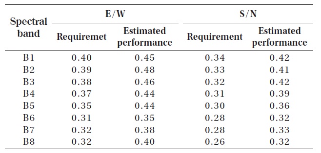
Predicted GOCI MTF performance at Nyquist frequencybefore launching (Herve et al. 2009).
the GOCI on-orbit MTF measurements for the three study cases. The conclusions are presented in Section 4.
Factors in the space environment, such as launch vibration and thermal loading, can change the resulting image quality (Holst 2000, Viallefont & Leger 2010). The on-orbit MTF performance assessment is a crucial step to determine whether the target optical system performance has been achieved in real instrument operation. The MTF performance can be estimated from the measured image products considering MTF degradation factors with the following equation (Manjunath 2003).

In Eq. (1), MTFtot refers to the final MTF from measured images, while MTFopt, MTFdet, MTFmot, MTFelec, MTFatm are MTF from the optical performance, detector performance, sensor operation effect, electronic noise and atmospheric effect, respectively.
Prior to the GOCI launch, the on-orbit MTF performance
[Table 2.] Comparison of MTF assessment calculation methods.

Comparison of MTF assessment calculation methods.
for each spectral band was predicted in both E/W and S/N directions as shown in Table 1. The estimated MTF performance at Nyquist frequency was computed with Eq. (2) as follows,


where MTFmeasured is measured as static MTF in the thermal vacuum environment, MTFsmearing is calculated from Eq. (2-2), kS = 1.2 and dLOS = 5.1μ m. Straylightmargin to reduce the overall starylight level was determined to be about 6.5% (Herve et al. 2009).
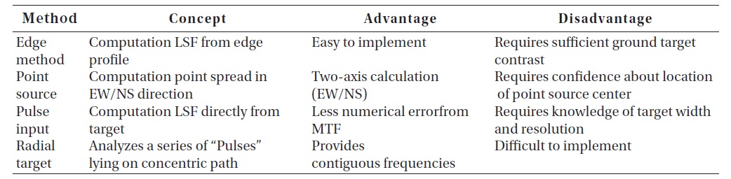
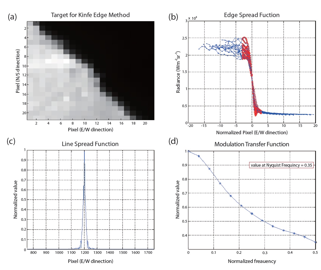
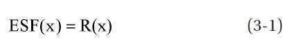
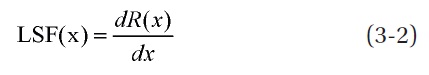
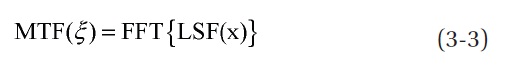
We used the knife-edge method,which is one of the widely used methods (Carnahan & Zhou 1986, Maeda et al. 1987, Choi 2002), and the point source method, as shown in Table 2. Edge spread function (ESF(x)) is defined by radiance (R) at pixel positions(x) in Eq. (3-1), line spread function (LSF(x)) of the system is computed by a simple discrete differentiation of the ESF as shown in Eq. (3-2). MTF (ξ) is obtained by Fourier transforming LSF.
In Fig. 3, considering the radiance recorded on the detector,the first step is to select the edge target. The target edges must have clear contrast differentiation in the edge boundary. When selecting such edges’ target area, nearby objects were trimmed out for noise reduction. The second step is to use the line profiles across the edge and to fit the
ESF as shown in Eq. (3-1). Its line profile data is the radiance read from each detector pixel position. Since the radiance at each pixel expresses the mixed radiance between land and sea, the interpolation technique was used to obtain 10 radiance data between adjacent pixel readings to eliminate the effects of the coastline environment from the measured radiance.
The third step is to make the LSF by taking the numerical derivative of the equally spaced ESF samples as shown in Eq. (3-2). In the last step, MTF is obtained by performing a Fast Fourier transform (FFT) of the resulting LSF as shown in Eq. (3-3), and normalizing its magnitude to 1 at the zero spatial frequency. In the case of the GOCI detector, pixel size is 14.81 μm in E/W direction, and 11.53 μ m in S/N direction, so the Nyquist frequency is calculated to 33.8mm-1 in E/W direction, and 43.4 mm-1 in S/N direction. We compare the case study results in terms of MTF at the Nyquist frequency.
This method uses point spread function (PSF) defined by Eq. (4).
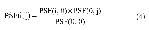
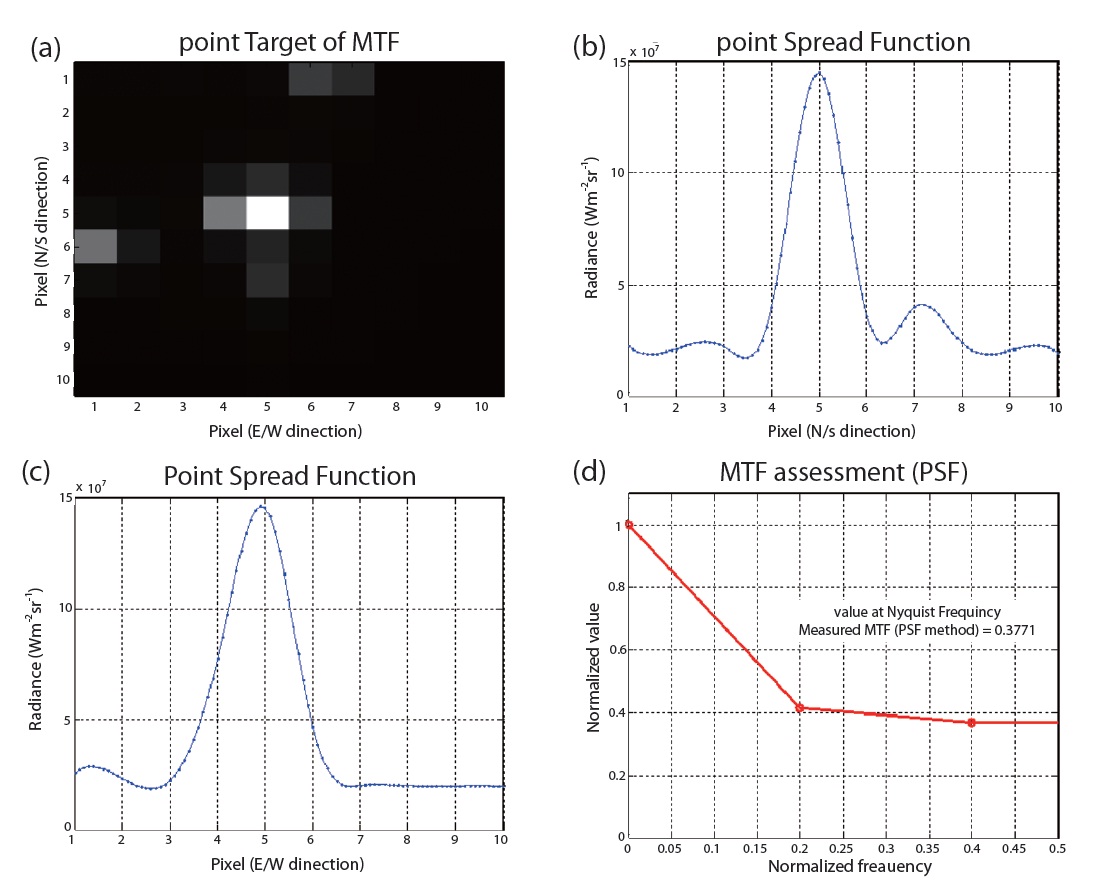
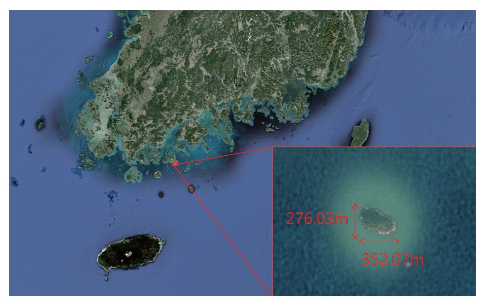
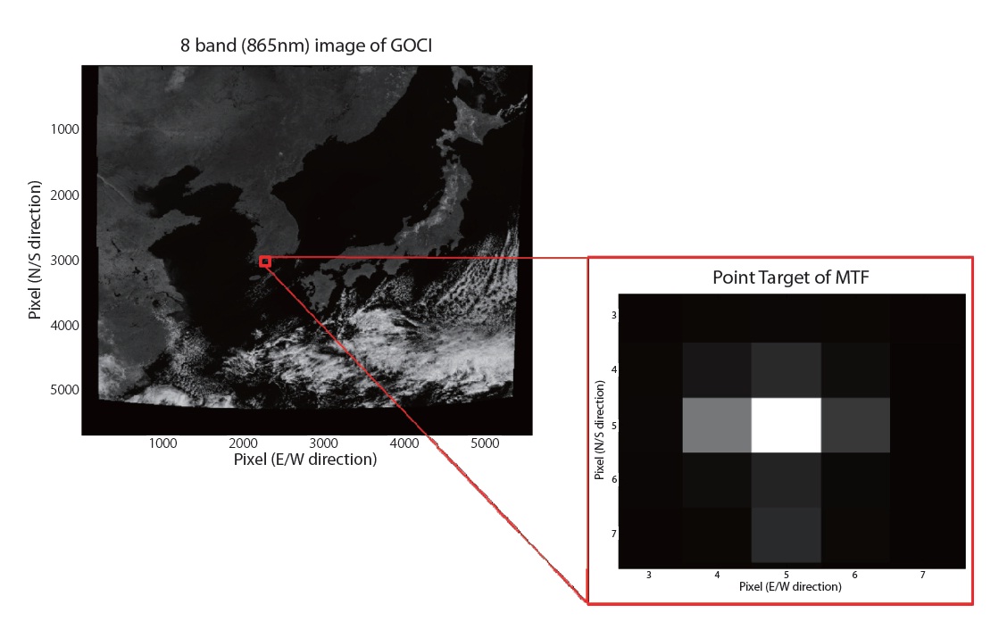
where PSF(i,j) is point spread function at an arbitrary pixel position (i, j), PSF (i,0) and PSF (0,j) are the 1-D LSF in horizontal and vertical direction respectively, and PSF (0,0) is obtained at the center position (Hwang et al. 2008). Using a powerful light source or lamp on the ground or a bright star source for a space telescope (Leger et al. 1994, Lee 2010), PSF can be acquired from the image with Eq. (4)(Hwang et al. 2008). The basic concept of the point source method is to use the FFT of blurred PSF that is similar to the LSF in the knife-edge method. We used GOCI L1B level data where small islands tens of metersor a hundred meters in size are removed due to its signal being engulfed by the surrounding ocean signal. An island target of 400m in size, corresponding to 352.07m in E-W direction and 276.03m in N-S direction, was selected for the MTF evaluation as shown in Fig. 4. PSF of the target island imagewas calculated with the same procedure as the knife-edge method.
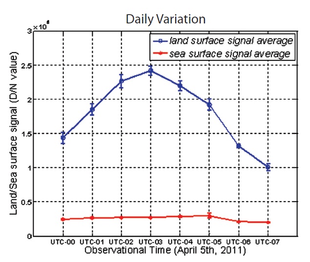
First, the on-orbit GOCI MTF performance was computed for a clear image taken at UTC-03 April 5th, 2011. MTF for 8 images obtained from UTC-00 to UTC-07 April 5th, 2011 was then also derived to check the hourly MTF variation. The monthly MTF variation was estimated with 4-days-images (in between Sep 15th, 2010 and May 17th, 2011) representing 3 seasons.
3.1 MTF Evaluation for Three Target Areas
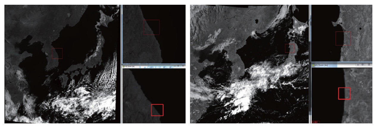
GOCI data processing uses the 8th band (865 nm), which serves as a reference wavelength for correction of atmospheric effects such as Rayleigh scattering, Mie scattering and aerosol. Therefore, using the 8th band image, the day and night time target images are selected with two conditions 1) i.e. smaller atmospheric effects (clear sky), 2) radiance standard deviation under 1% for average radiance of each target area (nearly uniform target). For East-West directional MTF evaluation, the knife-edge method uses shorelines with the clear linear edge occupying many pixel rows in order to obtain intensity profiles line by line. The point source method uses the aforementioned island and is capable of deriving MTF regardless of whether it is in N-S or E-W direction.
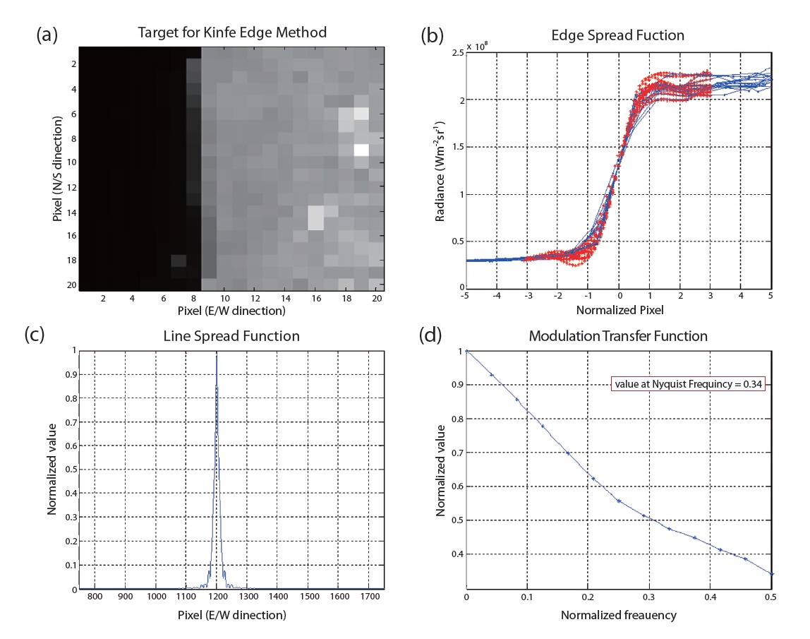
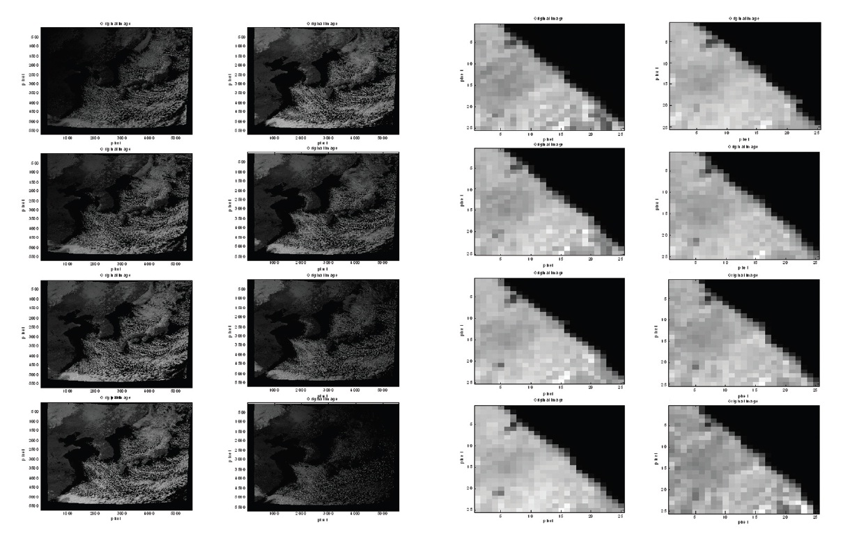
Table 3 shows the selected target image coverage used for knife-edge and point source methods. Some example coastline targets are illustrated in Fig. 5, whereas the point source target image of the GOCI 8th band is illustrated in Fig. 6. In addition, Figs. 7 and 8 show interim results in the MTF computation process with knife-edge method using the image taken at 03:15 UTC April 5th, 2011. In particular, Figs. 7a and 8a show edge targets used in the knife-edge method, and Figs. 7b and 8b show the combined edge
[Table 3.] MTF test target determination.
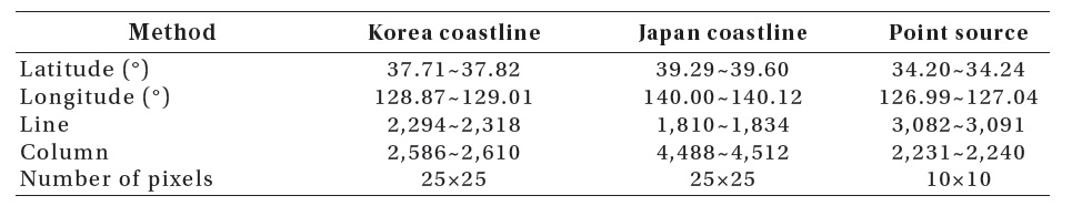
MTF test target determination.
profiles for pixel lines and the best fit line to the data. LSF was computed from differentiation of ESF as shown in Figs. 7c and 8c. The MTF estimation was then performed with the FFT, as shown in Fig. 7d and 8d. The resulting MTF from the Korea East Coastline edge target in Fig.7 is 0.35 at the Nyquist Frequency, and the result from the west coastline of Japan is 0.34. The MTF estimation with the point source
target is shown in Fig. 9a, and the computed MTF turns out to be 0.38 at Nyquist frequency as in Fig. 9b.
3.2 Trend Analysis for Daily MTF Variation
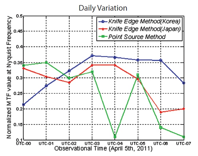
From the 8th spectral band images taken sequentially from UTC-00 to UTC-07 on April 5th, 2011, 8 target images used in the knife-edge method are listed in Fig. 10. The images show the variation in radiance according to the solar zenith angle, and UTC-03 image is the brightest, as shownin Fig. 11. In Fig. 12, the estimated MTF using the Korean coastline shows that MTF from the UTC-03 image has the best performance, with the maximum radiance contrast between land and sea surfaces, as the sun elevation angle is the highest. We note that the MTF results from three different targets are slightly different but satisfy the requirement of 0.32, as in Table 1.
In the meantime, the radiance difference between land and sea may affect the daily MTF variation, as shown in Fig. 12. The measured MTF using Japan’s coastline at UTC-06,
and 07, using the same knife edge method, cannot satisfy the requirement, and may be affected by the atmospheric radiance noise from cloud and aerosol. We also note that the MTF results from the point source method using the images at UTC-04, 06, and 07 are contaminated by the pixel spacing noise (Leger et al. 1994).
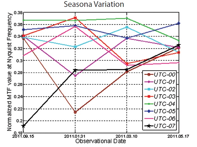
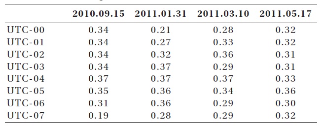
We compiled clear images taken over the time period of about 8 months from Sep 15th, 2010 to May 17th, 2011. The knife-edge method was then applied for every 8th spectral band image and we calculated the MTF at the Nyquist frequencyrespectively. The resulting MTF is shown in Table 4 and in Fig. 13.We note that there are some seasonal MTF variations in excess of the design MTF requirement. These can be interpreted as environmental (i.e. most likely atmospheric effects) degradation of the target image,rather than the optical system MTF variation. We also recognize that most results satisfy the MTF design requirement. Based
[Table 4.] MTF test target determination.

MTF test target determination.
on these results and interpretation, we are confident that the current GOCI operational MTF performance satisfactorily meets the resign requirement.
For the GOCI L1B level data, we have established the computational methods to monitor seasonal MTF trend for GOCI image products, and report based on the observational evidence of successful GOCI operation that the GOCI on-orbit MTF performance is well within the requirements. We used the coastline edge target and a small island as a point source for the 8th spectral band image obtained after geometric correction in the data pipeline procedure. Our on-orbit MTF estimation results show 0.32±0.04 on average, which satisfies the design requirement of 0.32. In addition, daily and seasonal variation test results illustrate that the GOCI MTF variation is stable within or close to the requirement. We believe that some MTF variations in excess of the requirement are caused by the target object condition or images rather than the optical system MTF.