Business management has entered a period in which supply chains compete with each other (Christopher, 1998). As firms head towards supply chain management (SCM), it becomes essential to measure the performance of the supply chain. Traditional performance measurement systems (PMSs) however, cannot adequately capture the complexity of supply chain performance for several reasons such as: They have been found to be lacking in a balanced approach to integrating financial and non-financial performance measures. They also fall short in terms of the systems thinking perspective, by which a supply chain must be viewed as the whole entity and measured widely across the whole. Traditional PMSs also lack effective techniques that can help supply chain managers to interpret the overwhelming amount of supply chain performance information (Chan
The literature on SCPM can be divided into the three major components of the PMS: performance models, supply chain metrics and measurement methods. The ‘per-formance model’ is a selected framework that links the overall performance with different levels of decision hierarchy to meet the objectives of the organization (Simatupang and Sridharan, 2002). The term ‘metric’ includes the definition of measure, data capture, and responsibility for calculation (Neely
A variety of performance models can measure supply chain performance according to different performance attributes (Beamon, 1999; Chan and Qi, 2003b; Chan 2003), processes (Gunasekaran
The literature concerning supply chain metrics suggests integrated measures (Bechtel and Jayaram, 1997; Brewer and Speh, 2000; Farris II and Hutchison, 2002; Novack and Thomas, 2004); identifies measures frequenttly used to guide supply chain decision making (Fawcett and Cooper, 1998; Harrison and New, 2002; and Bolstorff, 2003); invents new metrics (Lambert and Pohlen, 2001; Dasgupta, 2003); and cautions against measures of traditional logistics operations such as inventory turn (Lambert and Pohlen, 2001), logistics cost per unit (Griffis
When it comes to measurement methods, the analytic hierarchy process (Chan, 2003), the fuzzy set theory (Chan and Oi, 2003a) and a method used in the ABC inventory (Gunasekaran
In an attempt to resolve traditional PMS deficiencies, Chan and Qi (2003a) proposed an innovative measurement method that converts performance data from various measures into a meaningful composite index for a supply chain. The methodology developed is based on the fuzzy set theory to address the imprecision in human judgments. A geometric scale of triangular fuzzy numbers by Boender
Chan and Qi’s measurement method has made a significant contribution to SCM. Harland
The method is undoubtedly useful for SCM, yet there is room for improvement. First, supply chain practitioners may find it difficult to use Chan and Qi’s measurement method because of its very complex fuzzy set algorithm. Although the fuzzy logic-based approach is effective in making decisions and evaluations where preferences are not clearly articulated, managers who do not have the requisite academic expertise will be frustrated by the mathematical sophistication that it requires (Zanakis
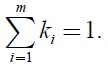
Second, it is important to recognize that Chan and Qi’s measurement approach has its roots in the weighted additive model of the multiattribute value theory (Keeney and Raiffa, 1976; Dyer and Sarin, 1979). Weights in such a model however, are scaling constants, which “do not indicate relative importance” (Keeney and Raiffa, 1976, p. 273). Weights as scaling constants rely on measurement scales (the ranges of measures being weighted). In general, the greater the range of performance for a particular measure, the greater the weight for the measure should be. If a particular measure has a small range between the worst and the best performance, this measure becomes irrelevant because it has no importance in discriminating between the worst and the best performance even though the evaluator may consider it an important measure
Third, the relationships between measurement scales and performance scores are somewhat
In view of the above limitations, a simple, flexible, and sound theoretical approach to SCPM is needed. Thus, the objective of this paper is to introduce an alternative measurement method that possesses such desirable features. Developed from the integration of the multiattribute value theory, the swing weighting method (von Winterfeldt and Edwards, 1986), and Saaty’s (1980) eigenvector procedure-the proposed measurement method is conceptually simple and comprehensible and both flexible and rigorous enough to cope with the human evaluation process.
The contributions of this paper are to: (1) develop a novel performance measurement method to contribute to the development of SCM, (2) point to an approach that can elicit weights in the additive aggregation model, (3) present an alternative modeling of judgments that permits both linear and non-linear value functions, and (4) provide an original case study to demonstrate the proposed approach.
In a subsequent section, the proposed performance measurement method for SCM and its development background are described. Next, details of a case study are provided. The paper ends with conclusions and discussions.
2. THE PROPOSED MEASUREMENT METHOD
Various measures have been proposed by several authors to capture many aspects of supply chain performance. Important measures of supply chain performance could be used collectively to depict the overall supply chain performance, and this evaluation could be administered through techniques typical to the field of multiple criteria decision analysis (MCDA). MCDA is a collection of formal approaches which take into account multiple criteria in helping individuals or groups to promote good decision making (Belton and Stewart, 2002). Common MCDA techniques embrace multiattribute value theory (MAVT), multiattribute utility theory (MAUT), the analytic hierarchy process (AHP), goal programming, and outranking methods (Belton and Stewart, 2002).
This study uses MAVT (Keeney and Raiffa, 1976; Dyer and Sarin, 1979) to provide a platform for integrating several measures of supply chain performance into a single indicator. MAVT is an approach that allows numerical scores (values) to represent the respondent’s preference for performance outcomes. The scores are usually derived by the construction of the respondent’s preference orderings or mathematical functions. Such a function is referred to as the ‘value function’ if the assessment of preference is not concerned with uncertainty. If the assessment involves risk and uncertainty, MAUT should be applied, and the function under uncertainty is referred to as the ‘utility function.’
In applying MAVT for SCPM, this study underscores the importance of modeling accurate value judgments. Accordingly, its scoring method allows non-linearity between performance outcomes and preference scores (values) to happen. In the literature, there has been a debate regarding the assumption of shapes of value functions. Von Winterfeldt and Edwards (1986) suggested that value functions should be linear or nearly linear if the problem (the performance model) has been well structured and if the appropriate scales have been selected. Belton and Stewart (2002), however, cautioned against the oversimplification of the problem by an inappropriate use of linear value functions because Stewart’s (1993, 1996) experimental simulations have showed that the results of MAVT models are very sensitive to inappropriate linearization.
A combination of non-linear value functions and the fuzzy set theory could lead to the daunting complexity of algorithm for practitioners and could create ambiguity regarding the interpretation of inputs. Although a decision support system (DSS) could be developed to help managers to take decisions without being frightened by model complexity, its modeling would be uneconomical since the model would take as long to build as the system it represented, and would be expensive to develop and control. Stewart (1992) addressed these potential limitations by suggesting that analysts apply value functions without fuzzy set theory to make it simple, easier to use, and transparent enough to generate further insights and understanding. The success of model implementation depends on good communication between the analyst and the decision maker (P?yh?nen and H?m?l?inen, 2000). Stewart (1992) stated that although attempts to apply fuzzy set theory to value functions may lead to effective models, doing so may enlarge the scope for misunderstanding between analysts and decision makers because the inputs required from the decision makers are not as straightforward as the unequivocal language of relative values. He further stated that the fuzziness of judgments is not an important matter in practical value function analyses because the decision maker can handle it by conducting sensitivity analyses. This study adopts Stewart’s (1992) suggestion by applying the value measurement theory without the fuzzy set theory.
We believe that the use of simple and understandable measurement methods contributes significantly to the important goal of improving the understanding and practice of SCPM. Likewise, research in MCDA has also called for the use of simple, understandable, and usable approaches for solving MCDA problems (Dyer
2.2 Weighted Additive Model of SCPM
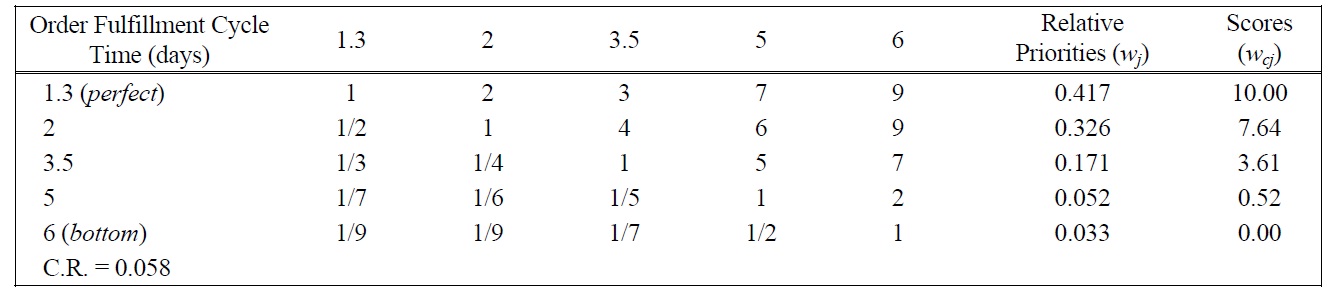
The weighted additive model of SCPM can be written as:
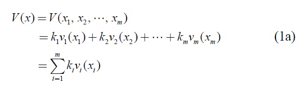
where the overall value (score)
Three assumptions must be kept in mind when applying the weighted additive model (Belton and Stewart, 2002). First, all measures have mutual preferential independence; the preference ordering in terms of one measure should not depend on the levels of performance on other measures. Second, the partial value functions are on an interval scale; only ratios of differences between values are meaningful. Third, weights are scaling constants; any method of assessing weights must be consistent with the algebraic meaning in the additive value function.
2.3 Assessing Weights of Measures
The weight parameters
where
The tradeoff procedure (Keeney and Raiffa, 1976) ? the standard method of eliciting weights for the additive model ? has the strongest theoretical foundation (Keeney and Raiffa, 1976; Schoemaker and Waid, 1982; Weber and Borcherding, 1993), yet this method is complicated and more likely to produce elicitation errors (Schoemaker and Waid, 1982; Borcherding
The swing weighting method would work as follows: First, the evaluator needs to consider a hypothetical situation in which all the metrics would be at their worst possible levels. The evaluator is allowed to move (swing) the most important metric to the best level and this metric would be assigned 100 points. The second most desirable attribute and the remaining attributes would then be respectively moved and assigned less than 100 points. The given points would then finally be normalized to sum to one to yield the final weights. The swing procedure will be explained in more detail when the case study is presented.
The value function reflects the evaluator’s preferences for different levels of achievement on the measurement scale. The first step in defining a value function is to identify its measurable scale. The second step is to establish the scale of the performance score so that the performance results from diverse measures can be combined into a meaningful figure. Next, the value function is constructed to convert the performance data into the performance score that reflects the extent to which the evaluator has a preference.
2.4.1 Interval Scale of Measurement
In the proposed method, the performance is assessed on the interval scale of measurement. To construct the interval scale, the evaluator specifies two end points of the scale. The end points can be defined in many ways (see for example, Belton and Stewart, 2002, § 5.2.1; von Winterfeldt and Edwards, 1986, § 7.3), but this study finds it useful to follow Chan and Qi’s measurement scale, set in terms of an interval [
2.4.2 Performance Score and its Scale
After the extreme points of the measurement scale have been specified, consideration must be given to the performance score, its scale, and how the score is to be assessed. The performance score is the logical number indicating the degree to which the particular performance satisfies the evaluator. Like Chan and Qi (2003a), this study sets the performance score on a scale of 0 to 10. The perfect point of the measurement scale is given a score of 10 and the bottom a score of 0. Other performance levels will receive intermediate scores which reflect their preferences relative to the extreme points.
2.4.3 Eigenvector Method for Assessing Value Functions
Although several techniques are available for developing value functions, the proposed method of eliciting values relies on the eigenvector method of the analytic hierarchy process (AHP) (Saaty, 1980). The AHP is an approach to multiple criteria decision analysis that has been extensively applied in modeling the human judgment process (Lee
The AHP is based on three principles: decomposition, comparative judgments, and the synthesis of priorities. The decomposition principle allows problem attributes to be decomposed to form a hierarchy. The principle of comparative judgments enables the assessment of pairwise comparisons of elements within a given level with respect to their parent in the adjacent upper level. The elements are compared according to the strength of their influence, which can be made in terms of importance, preference or likelihood. These pairwise comparisons are placed into comparison matrices to calculate the ratio scales that reflect the local priorities of elements. The principle of a synthesis of priorities allows decision makers to multiply the local priorities of the elements in a cluster according to the global priority of the parent element, thus producing global priorities throughout the hierarchy. In this paper, the proposed method of eliciting values is based on the second principle of the AHP.
Kamenetzky (1982) and Vargas (1986) have shown that it is possible to derive value functions from reciprocal pairwise comparisons and Saaty’s eigenvector method. The AHP-the eigenvector procedure in particular-is used to elicit values because of its unique characteristics. First, pairwise comparison judgments are easy to elicit because the evaluator can consider only two elements at a time. Second, the AHP allows for inconsistency in each set of pairwise judgments, and provides a measure of such inconsistency. Third, the redundancy of the information contained in the systematic pairwise comparisons contributes to the robustness of the value estimation (Kamenetzky, 1982). Finally, pair comparisons do not require making any assumption about the form of the value function.
Now we can take a closer look at the proposed method for developing partial value functions through the use of Saaty’s eigenvector method. To construct the partial value function, for each measure, the evaluator needs to establish the scale of measurement in terms of an interval [
The comparison between the pair of performance outcomes
[Table 1.] Mapping from Verbal Judgments into AHP 1-9 Scales.
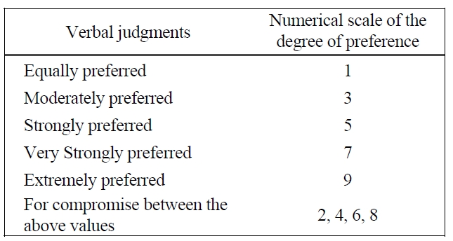
Mapping from Verbal Judgments into AHP 1-9 Scales.
The response, denoted by
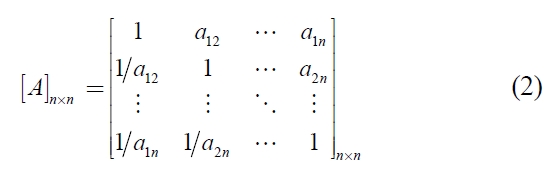
Local priorities are determined by solving the following matrix equation (Saaty, 1980):
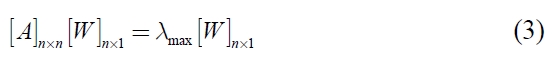
where [
A standard measure of the consistency of the evaluator’s judgment can be performed for each matrix by calculating a consistency ratio (
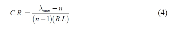
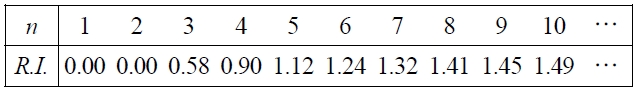
Based on simulations, the random index for various matrix sizes has been provided by Saaty (1980), as shown in Table 2. The acceptable
[Table 2.] The average random indices (R.I.).

The average random indices (R.I.).
The AHP in theory gives values on a ratio scale summed to one, whereas the MAVT scores in this study are on the 0-10 interval scale. To construct the partial value function, the priority orderings [
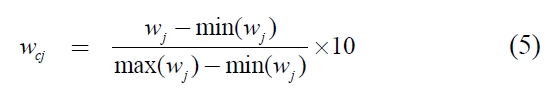
The
At this point, it is necessary to make certain that the value assessment process involves a fair number of
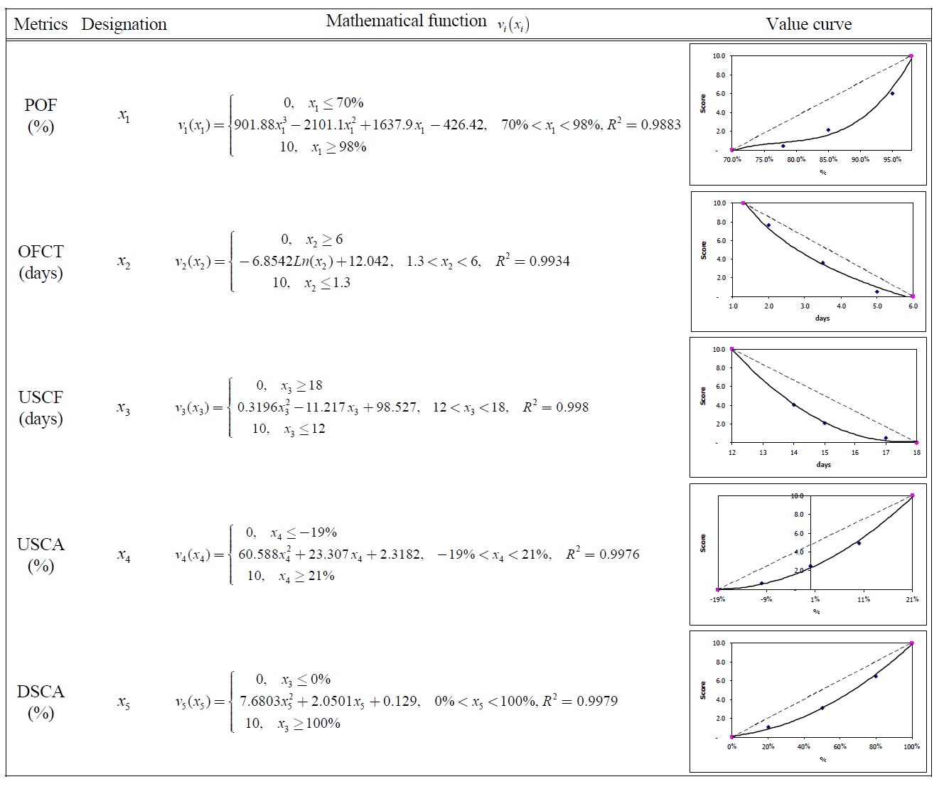
2.4.4 Value Curve Fitting
Having determined the five points and their corresponding scores, we can then graph and draw a curve through them. By drawing a line through the five individually assessed points, we can gain some idea about the shape and a possible functional form of the function. To standardize value analysis into a uniformly recognized form, we will fit a curve through these points to determine the corresponding equation for
It is very simple and easy for practitioners to use a Microsoft® Excel spreadsheet to conduct linear or nonlinear regression analyses since the spreadsheet does not require users to have an intimate understanding of the mathematics behind the curve fitting process. What is required from the users is the ability to select the correct type of regression analysis and the ability to judge the goodness of fit from the estimated function. By preparing an XY (Scatter) plot and using the ‘Add Trendline’ function- the value curve, its mathematical equation, and its Rsquared value can be obtained. As the assessment of a value function is subjective, a perfect representation is not necessary (von Winterfeldt and Edwards, 1986; Clemen, 1996). A smooth curve drawn through the assessed points as well as its equation should be an adequate representation of the value function with regard to a particular metric. The R-squared value provides an estimate of goodness of fit of the function to the data. A function is most reliable when its R-squared value is at or near 1.
After determining the swing weights, the partial value functions, and the current performance data of supply chain measures, the performance index can be computed. The performance index is determined by applying Equation 1a, multiplying the value score of a performance measure by the swing weight of that measure and then adding the resultant values. Because the values relating to individual measures have been assessed on a 0 to 10 scale and the weights are normalized to sum to 1, then the overall values of the supply chain performance index will lie on a 0 to 10 scale.
Note that supply chain performance is often assessed by managers working as a group whose information could
be utilized in the evaluation process. They normally come from various functions and management levels, and do not have equal expertise and knowledge. Since they may have different opinions, they may need to use an approach that allows them to aggregate individual judgments to obtain a group judgment. To resolve the differences, they may use mathematical aggregation to combine individual judgments. Mathematical aggregation methods involve such techniques as calculating simple averages and weighted averages of the judgments of individual evaluators. If some evaluators are better judges than others, the judgment aggregation process could adopt the weighted average method (Goodwin and Wright, 2004).
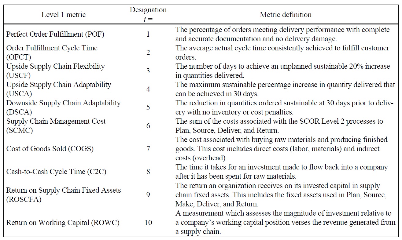
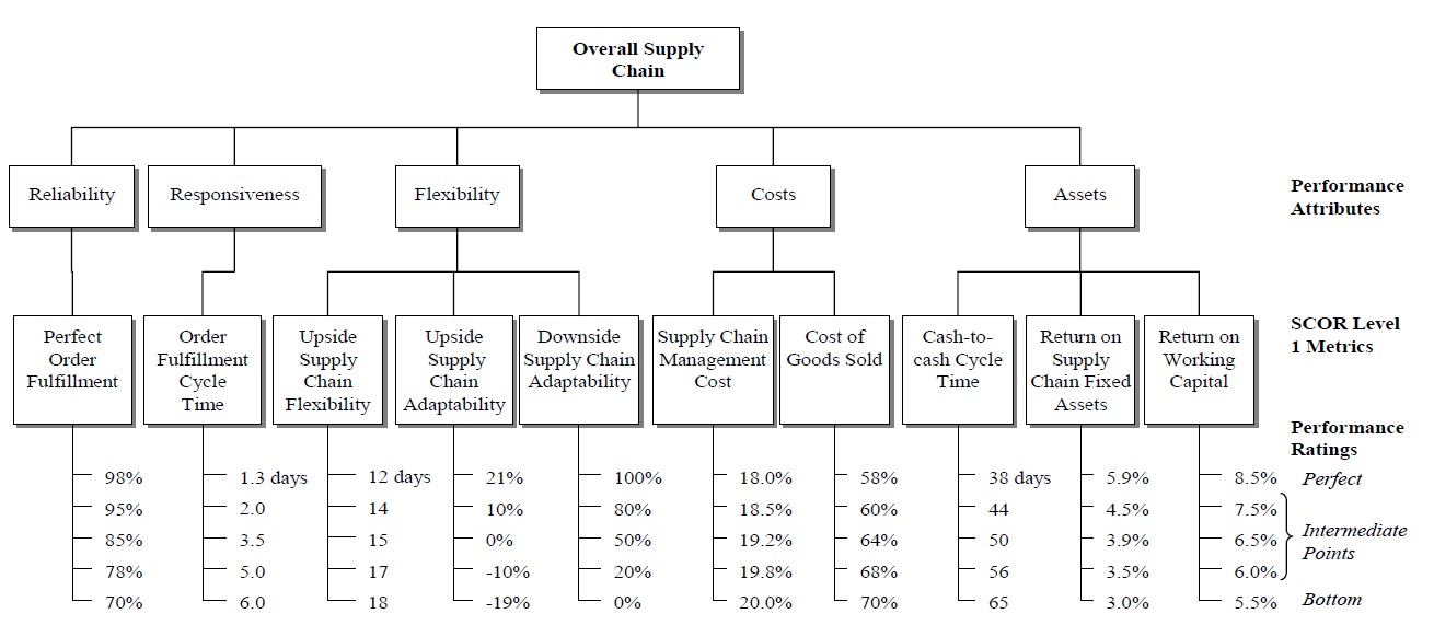
The case study selected to illustrate how the proposed measurement method can be applied looks at how one supply chain analyst evaluated the performance of a cement manufacturing supply chain in Thailand. Although multiple evaluators participated in our research, for the sake of brevity, we include only the assessment of one evaluator for this paper. The evaluator applied the Supply Chain Operations Reference (SCOR) model level 1 metrics (Supply-Chain Council 2006) to the performance model shown in Figure 1 (see Table 3 for metric definitions and abbreviations used in this study, and Table 4 for the monthly performance data). After examining the historical performance, the evaluator specified five performance ratings for every metric: two endpoints of the measurement scale and three arbitrary intermediate points. The weighted additive value function that depicted the supply chain performance was based on the SCOR level 1 metrics as shown in the following equation:
[Table 3.] Definitions of SCOR Level 1 Metrics.

Definitions of SCOR Level 1 Metrics.
[Table 4.] SCOR Level 1 Monthly Performance Data, 2006.
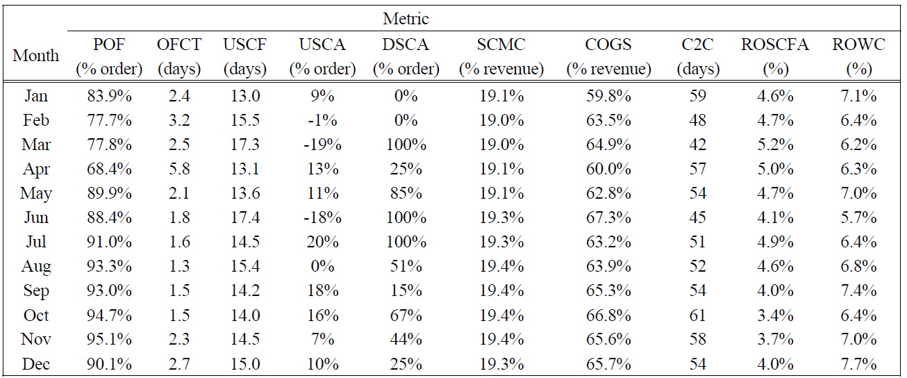
SCOR Level 1 Monthly Performance Data, 2006.
The first step in developing the compound value function
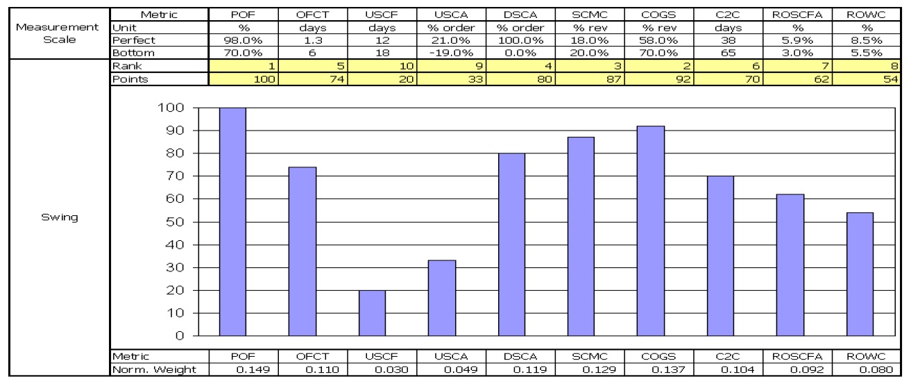
POF, the highest rank, was given a weight of 100. Other weights were assessed in the following series of steps. The evaluator was asked to compare a swing from the highest COGS to the lowest, with a swing from the lowest POF to the highest. After some thought, he decided that the swing in COGS was 92% as important as the swing in POF so COGS was given a weight of 92. Similarly, a swing from the worst to the best performance for SCMC was considered to be 87% as important as that of the worst to the best performance for POF, so SCMC was assigned a weight of 87. The swing procedure was repeated for the rest of the measures. The evaluator worked with a visual analogue scale like the one shown in Figure 2 to assess the relative magnitude of the swing weights. The ten weights obtained sum to 672, and since it is conventional to normalize them so that they add up to 1. Normalization is achieved by simply dividing each weight by the sum of weights (672). The normalized
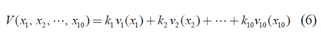
[Table 5.] Pairwise Comparison Judgments and Values of POF Performance Ratings.
Pairwise Comparison Judgments and Values of POF Performance Ratings.
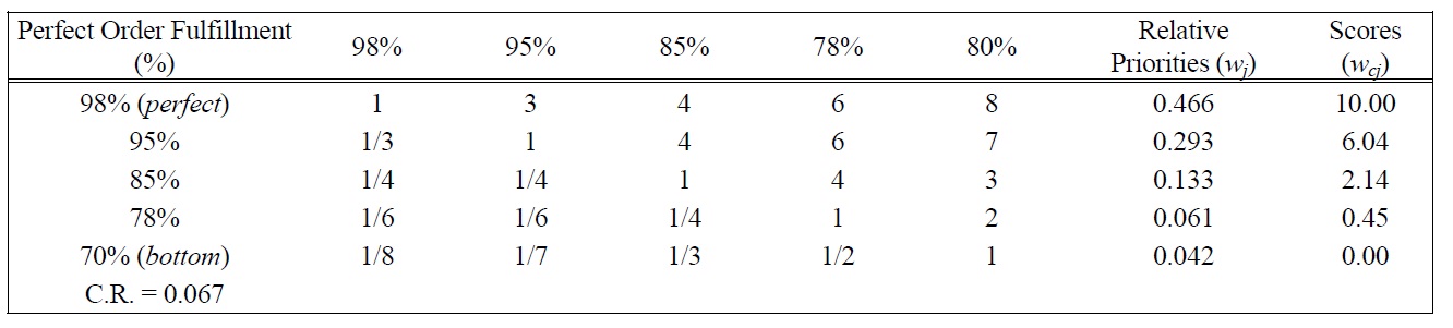
[Table 6.] Pairwise Comparison Judgments and Values of OFCT Performance Ratings.
Pairwise Comparison Judgments and Values of OFCT Performance Ratings.
swing weights are shown in Figure 2.
After eliciting the swing weights, the evaluator needed to develop the partial value functions
The partial value functions of ten measures are given in Table 15.
Based on the partial value functions and the swing
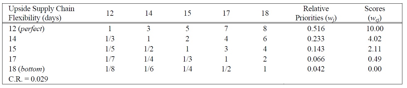
[Table 7.] Pairwise Comparison Judgments and Values of USCF Performance Ratings.

Pairwise Comparison Judgments and Values of USCF Performance Ratings.
[Table 8.] Pairwise Comparison Judgments and Values of USCA Performance Ratings.
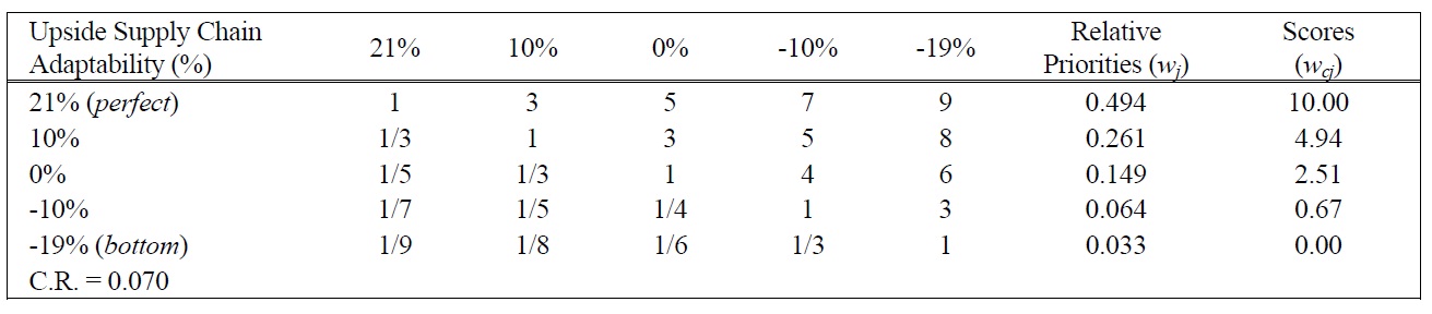
Pairwise Comparison Judgments and Values of USCA Performance Ratings.
[Table 9.] Pairwise Comparison Judgments and Values of DSCA Performance Ratings.
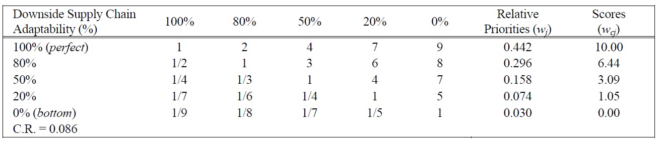
Pairwise Comparison Judgments and Values of DSCA Performance Ratings.
[Table 10.] Pairwise Comparison Judgments and Values of SCMC Performance Ratings.
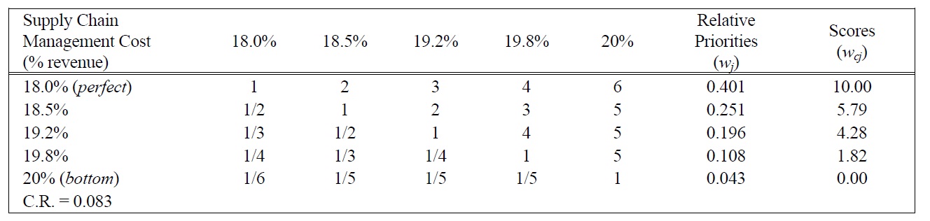
Pairwise Comparison Judgments and Values of SCMC Performance Ratings.
weights, the compound value function
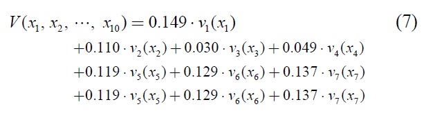
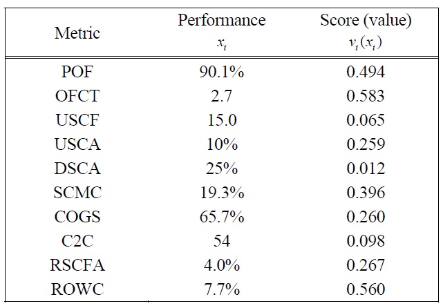
For the purposes of illustration, the performance data presented in Table 16 are from the sample month of December 2006. Using the partial value functions
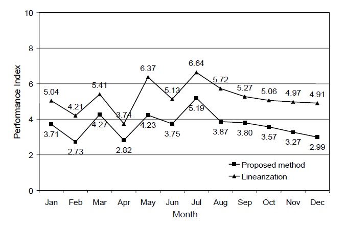
The number reveals that the overall supply chain performance was not very satisfactory. The supply chain manager would need to refine the supply chain operations to improve the performance. To monitor the progress of the supply chain, the monthly historical performance indices were calculated and plotted with the recent index as shown in Figure 3.
To compare the indices computed from the proposed
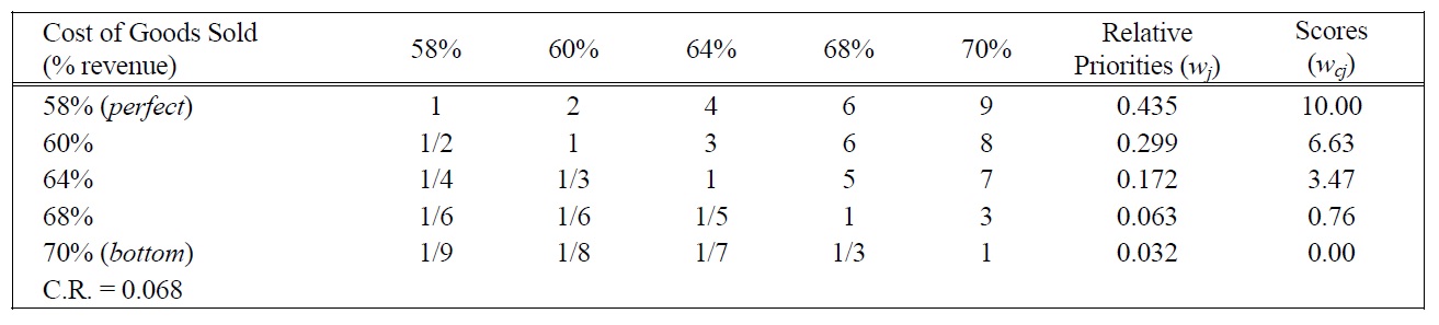
[Table 11.] Pairwise Comparison Judgments and Values of COGS Performance Ratings.

Pairwise Comparison Judgments and Values of COGS Performance Ratings.
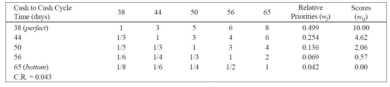
[Table 12.] Pairwise Comparison Judgments and Values of C2C Performance Ratings.

Pairwise Comparison Judgments and Values of C2C Performance Ratings.
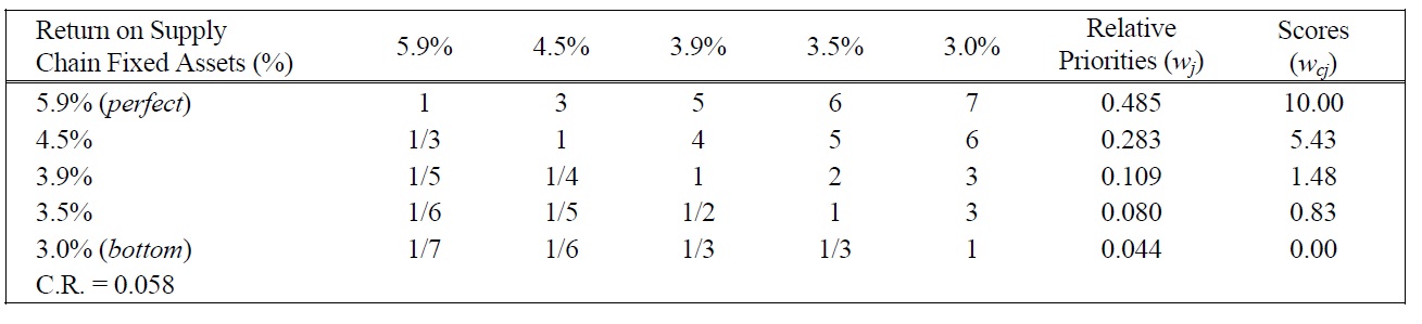
[Table 13.] Pairwise Comparison Judgments and Values of ROSCFA Performance Ratings.

Pairwise Comparison Judgments and Values of ROSCFA Performance Ratings.
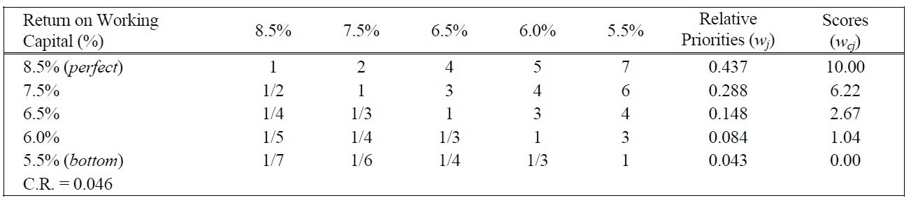
[Table 14.] Pairwise Comparison Judgments and Values of ROWC Performance Ratings.

Pairwise Comparison Judgments and Values of ROWC Performance Ratings.
measurement method with those whose value functions are linear by default, all the partial value functions were then assumed to be linear with respect to their bottom and perfect values, whereas the swing weights remained the same. By the default assumption of linearity, its resulting performance indices could be calculated and depicted as shown in Figure 3 to compare with those whose value functions would permit non-linearity.
From the figure one can see that the linearization indices were systematically higher than their counterparts. The average PI score assuming linearity was 5.21, whereas the average PI of the proposed method was 3.68.
There is a significant difference (15.2%) in terms of values between the average results of the two methods with respect to the ten-point scale. Since the two methods use the same set of performance data and swing weights, the difference was mainly attributed to the value curves. The finding of this case study supported evidence from the MCDA literature by showing how the default assumption of linearity can have a significant impact on the measurement result.
The proposed method’s value functions were mostly convex. Given the same measurement scale, linear functions map the performance outcomes into the higher performance scores, compared to those mapped by convex functions. This finding has an implication to the choice of value functions in real measurement problems. In practical terms, convex curves are more likely to motivate people to improve or maintain high performance because if they do not do so, they could earn extremely low marks for the measurement results. The overestimation of the
[Table 15.] Partial Value Functions for SCOR Level 1 Metrics.

Partial Value Functions for SCOR Level 1 Metrics.
[Table 16.] Performance of the supply chain of the case study, December 2006.

Performance of the supply chain of the case study, December 2006.
measurement results could not only lower the motivation for upgrading the performance but could also send a mis-
[Table 151.] Partial Value Functions for SCOR Level 1 Metrics (Cont.).
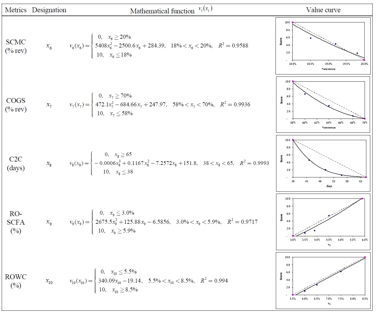
Partial Value Functions for SCOR Level 1 Metrics (Cont.).
leading signal to managers regarding the sense of urgency to improve the performance.
Chan and Qi (2003a) proposed the measurement and aggregation algorithm based on fuzzy sets and linear value functions to calculate the performance index for the supply chain. Although the measurement method is helpful in analyzing supply chain performance, the fuzzy set techniques can be quite complex due to the considerable number of calculations that are required. At the same time, it may produce defective weights because their meanings are not consistent with the weights in additive models. Moreover, the linearization of partial value functions can lead to a misleading performance index. To resolve these issues, this paper develops a user-friendly alternative measurement approach whose weighting parameters are pertinent to scaling constants in the additive model. The method developed is applicable to both linear and nonlinear value functions.
The proposed measurement method is presented based on the integration of the multiattribute value theory and the eigenvector method of the analytic hierarchy process and a real-world case study is provided. The weighted additive model is used to aggregate the performance information because it is the most widely used model. The measurement method relies on the swing weights of the supply chain metrics and on the eigenvector procedure for building partial value functions. The swing weighting method is applied because it produces weights compatible with weights in additive models. The eigenvector method provides a simple and useful tool in modeling both the linearity and non-linearity of value judgments. Once this method is fully applied, all the supply chain performance information can be aggregated into the overall performance index. As the performance index is formulated as a compound function of quantitative SCM measures, it can facilitate quantitative SCM research that investigates supply chain modeling and optimization.
The case study shows how the default assumption of linearity can affect the measurement result. It is advisable therefore, to allow non-linearity to take place when modeling human preference. Adopting non-linearity involves additional efforts: identifying additional anchor points, conducting pairwise comparisons, and performing additional calculations and regression analyses. It is, however, worth all the effort to do so not only to guard against obtaining misleading performance indices but also to understand the current performance situation and attitudes reflected in value functions.
The proposed measurement method has several advantages. First, it is flexible because it can handle both linearity and non-linearity. Second, the method is userfriendly because it is made up of simple and understandable MCDA tools. Belton and Stewart (2002) stated that the transparency, simplicity and user-friendly aspects of both the simple additive model and the AHP account for their widespread popularity. The proposed method shares these characteristics.