This paper focuses on three very similar evolutionary algorithms: genetic algorithm (GA), particle swarm optimization (PSO), and differential evolution (DE). While GA is more suitable for discrete optimization, PSO and DE are more natural for continuous optimization. The paper first gives a brief introduction to the three EA techniques to highlight the common computational procedures. The general observations on the similarities and differences among the three algorithms based on computational steps are discussed, contrasting the basic performances of algorithms. Summary of relevant literatures is given on job shop, flexible job shop, vehicle routing, location-allocation, and multimode resource constrained project scheduling problems.
Evolutionary methods for solving NP-hard optimization problems have become a very popular research topic in recent years. Among the many methods proposed, the three that are very similar and popular are the genetic algorithm (GA), particle swarm optimization (PSO), and differential evolution (DE). While GA is more well-established because of its much earlier introduction, the more recent PSO and DE algorithms have started to attract more attention especially for continuous optimization problems. While many papers were published based on these algorithms, most assessments are made empirically with specific cases on a particular application domain, and the two key performance indicators commonly used for comparison are the solution quality and solution time. Some example comparison studies include Hassan
This paper attempts to make a general qualitative comparison of the three evolutionary algorithms based on two aspects of a good metaheuristic algorithm, i.e., diversification and intensification. The observation will be focused on the elements of operations required and their effects on the diversification and intensification capabilities of each algorithm.
The paper is organized as follows. A general evolutionary algorithm is described at the conceptual level to highlight the common elements in all the evolutionary algorithms. The three targeted evolutionary algorithms are then described in turn in subsequent sections. Similarities and differences among the algorithms are discussed and highlighted. Finally, some reviews of literature that contain direct comparison of the algorithms are summarized.
2. GENERAL STEPS OF EVOLUTIONARY METHOD
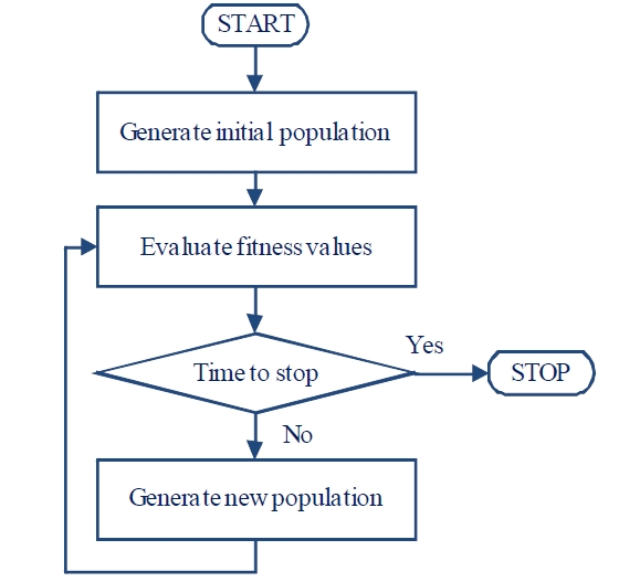
There are three main processes in all evolutionary algorithms. The first process is the initialization process where the initial population of individuals is randomly generated according to some solution representation. Each individual represents a solution, directly or indirectly. If an indirect representation is used, each individual must first be decoded into a solution. Each solution in the population is then evaluated for fitness value in the second process. The fitness values can be used to calculate the average population fitness or to rank the individual solution within the population for the purpose of selection. The third process is the generation of a new population by perturbation of solutions in the existing population. The three key processes are applied as shown in Figure 1. For a more recent in depth discussion of evolutionary algorithm, see Yu and Gen (2010).
As shown in Figure 1, after initialization, the population is evaluated and stopping criteria are checked. If none of the stopping criteria is met, a new population is generated again and the process is repeated until one or more of the stopping criteria are met. A stopping criterion may be static or dynamic. For example, a static stopping criterion may allow an algorithm to run for a fixed number of iterations. An example of a dynamic stopping criterion is to repeat the process until the top-
In using the evolutionary algorithm to solve optimization problems, the first important task is to determine how the solution can be represented according to the elements or terminology of the specific evolutionary algorithm. The processes for initialization and generation of new population may produce infeasible solutions. It is very important to choose a solution representation that is more likely to produce feasible solutions. This is a common design consideration for all evolutionary algorithms.
The solution representation can be a direct or an indirect one. The main design consideration is to ensure that each individual generated can always be decoded into a feasible solution. For a complex problem, indirect representation is often used along with a decoding procedure to convert the indirect solution representation into a feasible solution. Once the solution is decoded, the fitness function can be evaluated.
In addition to the solution representation, two common parameters that must be determined initially are the population size and the maximum number of iteration. The choices of values of these two parameters have major influence on the solution quality and solution time, and in practice, these values are almost always determined empirically through pilot runs.
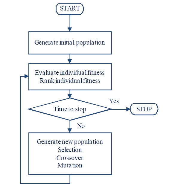
Although GA started much earlier than 1975, Holland (1975) is the key literature that introduced GA to broader audiences. The flowchart of the genetic algorithm is given in Figure 2.
The main idea of GA is to mimic the natural selection and the survival of the fittest. In GA, the solutions are represented as chromosomes. The chromosomes are evaluated for fitness values and they are ranked from best to worst based on fitness value. The process to produce new solutions in GA is mimicking the natural selection of living organisms, and this process is accomplished through repeated applications of three genetic operators: selection, crossover, and mutation. First, the better chromosomes are selected to become parents to produce new offspring (new chromosomes). To simulate the survivor of the fittest, the chromosomes with better fitness are selected with higher probabilities than the chromosomes with poorer fitness. The selection probabilities are usually defined using the relative ranking of the fitness values. Once the parent chromosomes are selected, the crossover operator combines the chromosomes of the parents to produce new offspring (perturbation of old solutions). Since stronger (fitter) individuals are being selected more often, there is a tendency that the new solutions may become very similar after several generations, and the diversity of the population may decline; and this could lead to population stagnation. Mutation is a mechanism to inject diversity into the population to avoid stagnation. More detailed discussions can be found in the more classic reference by Holland (1975), Goldberg (1989) and the more recent reference by Gen and Cheng (1997), and Gen
In addition to the population size and the maximum number of iterations, several decisions on parameters must be made for GA. The first set of decisions is the selection method and the probability assignment mechanism that is based on fitness. Different selection methods may require different mechanisms for probability assignments to ensure the balance of the diversity of the new population and the improvement of solutions. There are many proposed selection methods in literature, but the two most popular ones are the roulette wheel selection and tournament selection. Crossover method and crossover probability are the second set of decisions to be made. Many crossover methods are reported in literature since simple crossover methods have the tendency to produce infeasible or unusable chromosomes for many complex optimization problems. Finally, the mutation method and mutation probability must be selected as they may help to maintain the diversity of the population by injecting new elements into the chromosomes. In general, these three sets of decisions are set empirically using pilot runs.
There are many software implementations of GA available from various sources. A more general implementation of GA is the C++ GALib by Wall (1996) that allows the user to work at the source code level to apply GA with any representations and any genetic operators. The GALib classes provide the framework, and the user can solve a problem using GA by simply defining a representation, genetic operators, and objective function. Other software packages for GA are also available in EXCEL Solver (Frontline Solvers, http://www.solver.com/), and MatLab (http://www.mathworks.com/products/gads/).
4. PARTICLE SWARM OPTIMIZATION
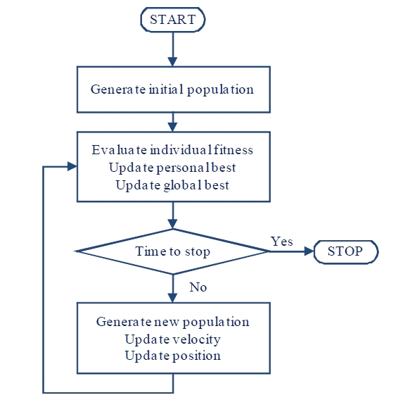
In 1995, a paper on PSO was presented at the Congress on Evolutionary Computation (Kennedy and Eberhart, 1995). This landmark paper triggered waves of publications in the last decade on various successful applications of PSO to solve many difficult optimization problems. It is very appealing because of the simple conceptual framework and the analogy of birds flocking facilitated conceptual visualization of the search process. The basic PSO algorithm is shown in Figure 3.
In PSO, a solution is represented as a particle, and the population of solutions is called a swarm of particles. Each particle has two main properties: position and velocity. Each particle moves to a new position using the velocity. Once a new position is reached, the best position of each particle and the best position of the swarm are updated as needed. The velocity of each particle is then adjusted based on the experiences of the particle. The process is repeated until a stopping criterion is met.
Similar to GA, the first process of PSO is initialization whereby the initial swarm of particles is generated. The concept of solution representation is also applied here in very much the same manner as GA. Each particle is initialized with a random position and velocity. Each particle is then evaluated for fitness value. Each time a fitness value is calculated, it is compared against the previous best fitness value of the particle and the previous best fitness value of the whole swarm, and the personal best and global best positions are updated where appropriate. If a stopping criterion is not met, the velocity and position are updated to create a new swarm. The personal best and global best positions, as well as the old velocity, are used in the velocity update.
As mentioned earlier, the two key operations in PSO are the update of velocity and the update of position. The velocity is updated based on three components: the old velocity (inertia or momentum term), experience of an individual particle (cognitive or self learning term), and experience of the whole swarm (group or social learning term). Each term has a weight constant associated with it. For basic PSO algorithm, the number of required constants is three.
It should be noted that PSO algorithm does not require sorting of fitness values of solutions in any process. This might be a significant computational advantage over GA, especially when the population size is large. The updates of velocity and position in PSO also only require a simple arithmetic operation of real numbers.
Software implementation of PSO algorithm is now available in various forms, ranging from black-box to user modifiable source code. One software library for PSO algorithm that follows the design principle of GALib is named ET-Lib, Nguyen
DE was proposed about the same time as PSO by Storn and Price (1995) for global optimization over continuous search space. Its theoretical framework is simple and requires a relatively few control variables but performs well in convergence. For some unknown reason, DE caught on much slower than PSO but has lately been applied and shown its strengths in many application areas (Godfrey and Donald, 2006; Qian
In DE algorithm, a solution is represented by a D-dimensional vector. DE starts with a randomly generated initial population of size N of D-dimensional vectors. In DE, the values in the D-dimensional space are commonly represented as real numbers. Again, the concept of solution representation is applied in DE in the same way as it is applied in GA and PSO.
The key difference of DE from GA or PSO is in a new mechanism for generating new solutions. DE generates a new solution by combining several solutions with the candidate solution. The population of solutions in DE evolves through repeated cycles of three main DE operators: mutation, crossover, and selection. However, the operators are not all exactly the same as those with the same names in GA.
The key process in DE is the generation of trial vector. Consider a candidate or target vector in a population of size N of D-dimensional vectors. The generation of a trial vector is accomplished by the mutation and crossover operations and can be summarized as follows. 1) Create a mutant vector by mutation of three randomly selected vectors. 2) Create trial vector by the crossover of mutant vector and target vector.
First, a mutant vector is generated by combining three randomly selected vectors from the population of vectors excluding the target vector. This combining process of three randomly selected vectors to form the mutant vector
The second step is to create the trial vector by performing crossover between the mutant vector and the target vector. There are two commonly used crossover methods in DE: binomial crossover and exponential crossover. Here, the crossover probability must be specified. A small crossover probability leads to a trial vector that is more similar to the target vector while the opposite favors the mutant vector.
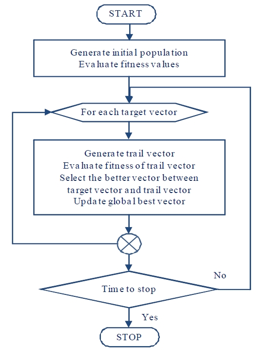
After the trial vector is formed for a given target vector, selection is done to keep only one of the two vectors. The simple criterion is to keep the vector with better fitness value. In other words, the target vector will survive if the trial vector has poorer fitness. Otherwise, the trial vector replaces the target vector immediately and becomes eligible for selection in the formation of the next mutant vector. This is an important difference since any improvement may affect other solutions without having to wait for the whole population to complete the update. The basic flow of a DE algorithm is summarized in Figure 4.
As shown in Figure 4, the first process is the generation of a population of new solutions called vectors. Each vector in the population is evaluated for fitness value. Each vector takes turns as a candidate or target vector, and for each target vector, a trial vector is formed. The selection process simply chooses between the target vector and trial vector, i.e., the winning vector between the trial vector and the target vector survives into the next round while the losing vector is discarded.
Several observations are made here. First, since a new solution would be selected only if it has better fitness, the average fitness of the population would be equal or better from iteration to iteration. Any improvement in the solution is immediately available to be randomly selected to form a mutant vector for the next target vector. This is different from GA and PSO where an improvement would take effect only after all the solutions has completed the iteration.
In contrast with GA where parent solutions are selected based on fitness, every solution in DE takes turns to be a target vector (one of the parents), and thus all vectors play a role as one of the parents with certainty. The second parent is the mutant vector which is formed from at least three different vectors. In other words, the trial vector is formed from at least four different vectors and would replace the target vector only if this new vector is better than the target vector; otherwise, it would be abandoned. This replacement takes place immediately without having to wait for the whole population to complete the iteration. This improved vector would then immediately be available for random selection of vectors to form the next mutant vector.
There are several variations of the DE proposed such as those including the best vector in the formation of the mutant vector or to use more vectors in the process. For more detailed information on the DE algorithm, see Price
In the three algorithms discussed above, one of the key differences is in the mechanism to produce a new population of solutions via perturbation of solutions from the old population. These different mechanisms generate a population of solutions with different balance between intensification and diversification. This dynamic behavior of the population can be deducted from the basic perturbation method used in the creation of new solutions. This section discusses the three algorithms based on two aspects: intensification and diversification.
The discussion will be made algorithm by algorithm. Suppose that the same solution representation is used and the initial population is exactly the same. It should be noted that all evolutionary algorithms may require a decoding process and checking of constraints to ensure that the solutions are feasible.
For GA, the solutions are ranked based on the fitness values. The parents are selected based on probabilities that favor individuals with better fitness. The crossover operation produces offspring with parts taken from the parents and the solutions are more likely to be similar to the parents. Based on this observation, GA tends to generate solutions that are more likely to cluster around several “good” solutions in the population. The diversification aspect of GA is accomplished through the mutation operation that injects some “difference” into the solutions from time to time. The solution time of GA also increases non-linearly as the population size increases because of the required sorting.
For PSO, a new swarm of particles is generated via the velocity and position update equations. This ensures that all new particles can be much different than the old ones. Also, since the mechanism is based on the floating point arithmetic, it could generate any potential values within the solution space, i.e., the density of the solutions within the solution space may be much higher than those generated via GA. In other words, the solutions can be much closer to each other than solutions in GA. In addition, the best particle in the swarm exerts its oneway influence over all the remaining solutions in the population. This often leads to premature clustering around the best particle, especially if the fitness gaps are large.
Similar to PSO, since the mechanism to generate new solutions of DE is also based on the floating point arithmetic, the exploration ability of the population might be comparable to PSO, but the diversification is better because the best solution in the population does not exert any influence on the other solutions in the population. Furthermore, the mutant vector is always a solution that is not from the original population; therefore, the crossover operation in DE is always between a solution from the population and a newly generated one.
For any evolutionary algorithm, the solutions are gradually clustered around one or more “good” solutions as the search evolves. This clustering can be seen as the convergence of the population toward a particular solution. If the population clusters very quickly, the population may become stagnated and any further improvement becomes less likely.
6.1 The Effect of Re-Initialization
Among the three algorithms, PSO has a higher tendency to cluster rapidly and the swarm may quickly become stagnant. To remedy this drawback, several subgrouping approaches had been proposed to reduce the dominant influence of the global best particle. A much simpler and frequently used alternative is to simply keep the global best particle and regenerate all or part of the remaining particles. This has the effect of generating a new swarm but with the global best as one of the particles, and this process is called the re-initialization process. In GA, the clustering is less obvious, but it is often found that the top part of the population may look similar, and that re-initialization can also inject randomness into the population to improve the diversity. In DE, the clustering is the least and re-initialization has the least effect for DE.
6.2 The Effect of Local Search
In GA, the density of the population in the solution space is less, so it is often found that the GA operators cannot produce all potential solutions. A popular fix is the use of local search to see if a better solution can be found around the solutions produced by GA operators. The local search process is often time consuming, and to apply it over the whole population could lead to a long solution time. For PSO, the best particle has a dominant influence over the whole swarm, and a time saving strategy is to only apply local search to the best particle, and this can lead to solution improvement with shorter solution time. This strategy was demonstrated to be highly effective for job shop scheduling in Pratchayaborirak and Kachitvichyanukul (2011). This same strategy may not yield the same effect in DE since the best particle does not have a dominant influence on the population of solutions.
6.3 The Effect of Sub-Grouping
Sub-grouping is a simple strategy to delay premature clustering of solutions. Sub-grouping can be done either with homogeneous population or heterogeneous population. Homogeneous population refers to the fact that each solution in the population uses the same operators and the same parameters during the evolutionary process. Heterogeneous population allows solutions in different sub-group to use different operators and parameters, thus allow for more diverse search behavior. The use of sub-grouping of homogenous population to improve solution quality has been demonstrated in GA and PSO. This sub-grouping allows some groups of solutions to be freed from the influence of the dominant solutions, and thus the group may be searching in a different area of the solution space and improve the exploration aspect of the algorithms. For DE, the best particle has little influence on the perturbation process so it is rational to presume that sub-grouping with homogeneous population may have limited effect on the solution quality of DE. However, no research literature is found that addresses this issue. Pongchairerks and Kachitvichyanukul (2005) proposed a use of heterogeneous population in PSO to allow some fraction of the swarm
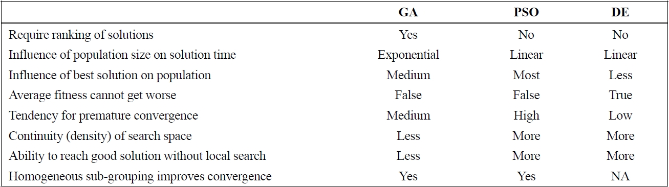
[Table 1.] Qualitative comparison of GA, PSO, and DE

Qualitative comparison of GA, PSO, and DE
to move by crossover with the best particle.
Dynamic change of population behavior can also achieve effects similar to the use of heterogeneous population. When more than one search strategies are included, the population can use the same search strategy as long as the solution continues to improve. If the solutions do not improve after some number of iterations, the population switches to use a different search strategy. Wisittipanich and Kachitvichyanukul (2012) applied strategy switching with DE for job shop scheduling problems.
The comparisons made in earlier sections are tabulated in Table 1. There are many research literatures that compare performances of these three evolutionary algorithms in solving some difficult optimization problems in various domains. The comparisons are often made indirectly since many researchers applied different solution representations in combination with various local search. Thus it is not so clear if the contributor to the algorithm performance is from the evolutionary algorithm or from the local search. The comparison is more comprehensive when benchmark problems are used with the same solution representation and the same number of function evaluations. Some recent references on successful applications of evolutionary algorithms for important combinatorial problems are summarized in Table 2.
[Table 2.] List of relevant literatures for various domains of combinatorial optimization
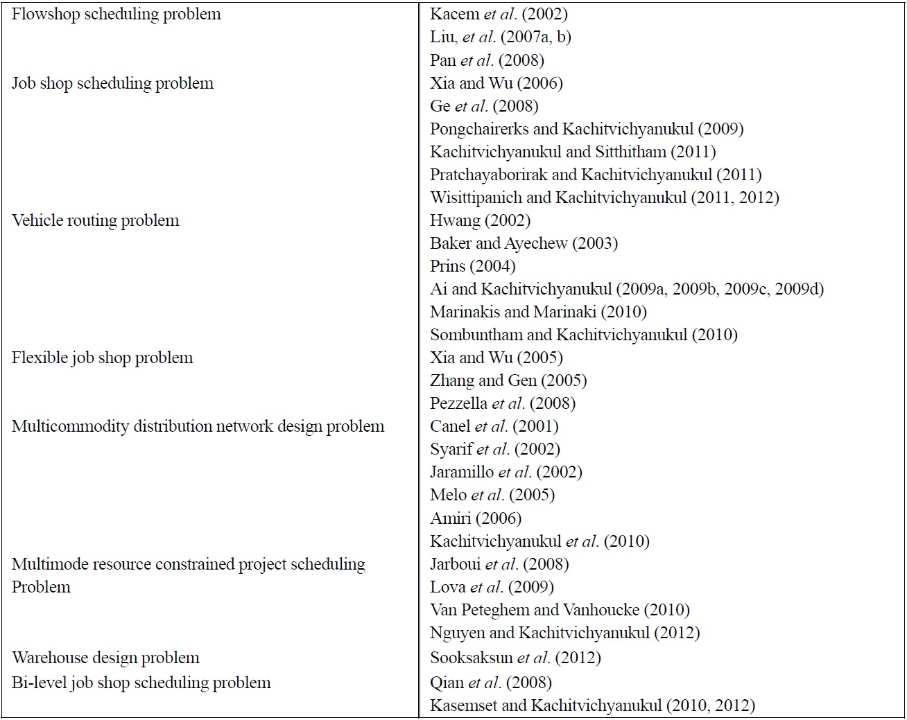
List of relevant literatures for various domains of combinatorial optimization