Lot sizing and shipment scheduling are two interrelated decisions made by a manufacturing plant and a third-party logistics distribution center. This paper analyzes a dynamic inbound ordering problem and shipment problem with a freight container cost, in which the order size of multiple products and single container type are simultaneously considered. In the problem, each ordered product placed in a period is immediately shipped by some freight containers in the period, and the total freight cost is proportional to the number of containers employed. It is assumed that the load size of each product is equal and backlogging is not allowed. The objective of this study is to simultaneously determine the lot-sizes and the shipment schedule that minimize the total costs, which consist of production cost, inventory holding cost, and freight cost. Because the problem is NP-hard, we propose three meta-heuristic algorithms: a simulated annealing algorithm, a genetic algorithm, and a new population-based evolutionary meta-heuristic called self-evolution algorithm. The performance of the meta-heuristic algorithms is compared with a local search heuristic proposed by the previous paper in terms of the average deviation from the optimal solution in small size problems and the average deviation from the best one among the replications of the meta-heuristic algorithms in large size problems.
Most manufacturing companies do not have a specialty of logistics functions. In order to obtain the benefit of shipping and warehousing costs, they strategically ally with a specialized third-party logistics (TPL) company for offering a wide range of services including: order fulfillment, inbound freight, warehousing, freight consolidation, outbound dispatching. They outsource the logistics operations to TPL company and concentrate on their core manufacturing operation.
Among the services provided by a TPL company, this paper focuses on the most important process is replenishing the multiple products by a number of freight containers at right time from manufacturers to the TPL warehouse. This process leads to managerial decision problems in determining replenishment lot-sizes and shipment schedule for each demand. For these problems the freight cost as well as the ordering and holding cost are considered. Since the replenishment orders are assumed to be shipped in containers to the warehouse, the freight cost is assumed to be proportional to the number of containers used. To solve this problem, this paper proposes an integrated optimization model of inbound ordering and outbound dispatching for single product in a TPL company.
The demand in this paper is assumed to be known, but dynamic over a discrete and finite time horizon. The production-inventory problem with the demand is called the dynamic lot-sizing model (DLSM), which has stemmed from the work of Wagner and Whitin (1958). Though there are a number of research results dealing with the DLSM, the majority of DLSMs have not considered any production-inventory problem incorporating shipment problem as well. These days, the issue of shipment scheduling for ordered products (or delivering orders) by a proper shipping freight container mode at right time becomes significantly important in production and distribution management because of the increasing fuel price.
Several studies have focused on various general costs and the capacitated resources as the extended works of the classical DLSM. Lippman (1969) studied two deterministic multi-period production planning models; monotone cost model and concave model. Florian
Anily and Tzur (2005) considered a dynamic model of shipping multiple items by capacitated vehicles. They presented an algorithm based on a dynamic programming approach. Van Norden and van de Velde (2005) dealt with a multiple product problem of determining transportation lot-sizes in which the transportation cost function has piece-wise linear as to a transportation capacity reservation contract. They proposed a Lagrangian relaxation algorithm to compute lower and upper bounds. Lee
In this paper, we propose three meta-heuristic algorithms to define the multi-product lot-size problem and shipment scheduling that minimize the total costs, which consist of ordering cost, inventory holding cost, and freight cost by generalizing the basic model of Kim and Lee (2012). The proposed heuristic algorithms are the first study in simultaneously determining multi-product lot-sizing problem and the shipment scheduling.
This paper is organized as follows. In the next section, the mathematical model of the problem is described. In Section 3, the properties of the optimal solution are characterized. Three meta-heuristic algorithms based on the optimal solution properties are described in Section 4. The computational results from a set of simulation experiments are presented in Section 5.
The following notations are defined to formulate the problem:
TH = the set of discrete time horizon, (t = 1, 2, …, T)
PD = the set of products, (i = 1, 2, …, M)
dti = amount demanded for product i in period t,
wi = volume of product i,
W = carrying capacity of a container,
St = ordering cost of product i in period t,
hti = unit inventory holding cost of product i from period t to period t+1,
F = unit freight cost of container,
xti = amount of product i ordered and shipped by container in period t,
zti = 1, if an order is incurred for product i in period t, and 0, otherwise,
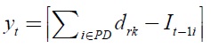
yt = number of containers used in period t (non-negative integer),
lti = inventory level of product i in period t
The objective of the problem is to determine (
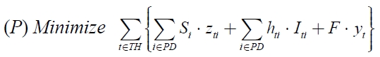


If we assume that all products have the same volume, the model (
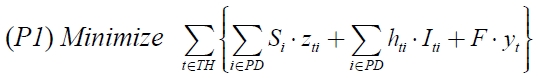
and (1), (3), (4), (5), and (6)
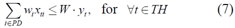
Constraint (2) ensures that the inventory level of each product in the current period balances the inventory level in the previous period, the ordering amount and the demand in the current period. Constraints (3) and (7) imply that the total ordering amount is restricted by the total carrying capacity associated with the number of containers used in the period. Constraint (4) ensures the relation between
3. OPTIMAL SOLUTION PROPERTIES
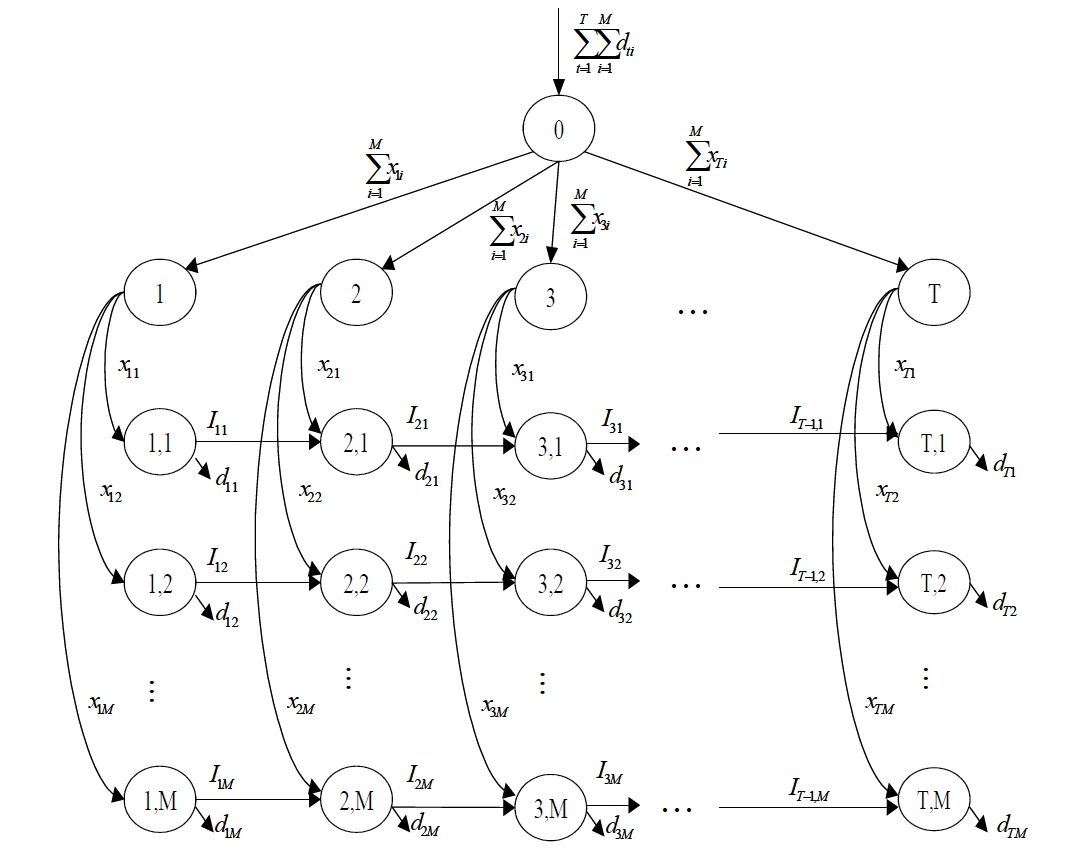
The mathematical model (
Here, the arcs in the aggregate flow are restricted by the capacities associated with the number of containers used whereas the arcs in the individual flow are not.
The optimal solution of the model (
In Figure 1, loops can be formed by two cases as follows. 1) Between the aggregate flow and the individual flow, for example, the loop can be formed by the sequences of nodes (0), (1), (1, 1), (2, 1), (2) and (0); 2) On the individual flows, for example, the loop can be formed by the sequences of nodes (1, 1), (1), (1, M), (2, M), (2), (2, 1), and (1, 1).
Ordering and shipment schedule satisfying the optimal solution property by Wagner and Whitin (1958),
(
Theorem 1:
Proof: Suppose that there exists the optimal solution which has two partial aggregate point between two consecutive inventory points for product
Theorem 2:
Proof: Suppose that there exists a feasible flow that satisfies the properties of Theorems 1 and 2, which has a loop formed by the sequences of nodes (1, 1), (1), (1, 2), (2, 2), (2), (2, 3), (3, 3), (3), (3, 1), (2, 1) and (1, 1) in Figure 1. Because arcs in the individual flow are not capacitated, there exists a positive loop formed by unsaturated arcs. This feasible flow is not an extreme flow. Therefore, the proof is completed.
Van Norden and van de Velde (2005) proved that the single level non-capacitated multi-product multi-period lot-sizing with transportation cost model is NP-hard in the strong sense. Hence, the problem (
In this section, we propose three meta-heuristics: a simulated annealing (SA) algorithm, a genetic algorithm (GA), and a self-evolution algorithm (SEA) based on the properties of Theorems 1 and 2.
For the solution representation of three meta-heuristic algorithms, a solution is defined as two dimensional array of (
In this representation,
Step 1: Set
Step 2: Let
Step 3: Set
Step 4: If
Step 5: If
then STOP. Otherwise,
Property 1: For the model
In this representation, one can easily find that the first nonzero value of
The GA, which has been widely used in solving various optimization problems for the last three decades, is a stochastic search algorithm based on the mechanism of natural selection and natural genetics. Being different from conventional search techniques, it starts with an initial set of (random) solutions called a population. Each individual in the population is called a chromosome, representing a solution to the problem at hand. The chromosomes are evaluated, using some measures of fitness. Generally speaking, the GA is applied to spaces that are too large to be exhaustively searched (Goldberg, 1989). In this paper, the chromosomes that have higher fitness value (lower objective function value) than the average fitness of current population make a potential parent pool and new chromosomes in the next generation are randomly selected from the parent pool or selected from the roulette wheel method.
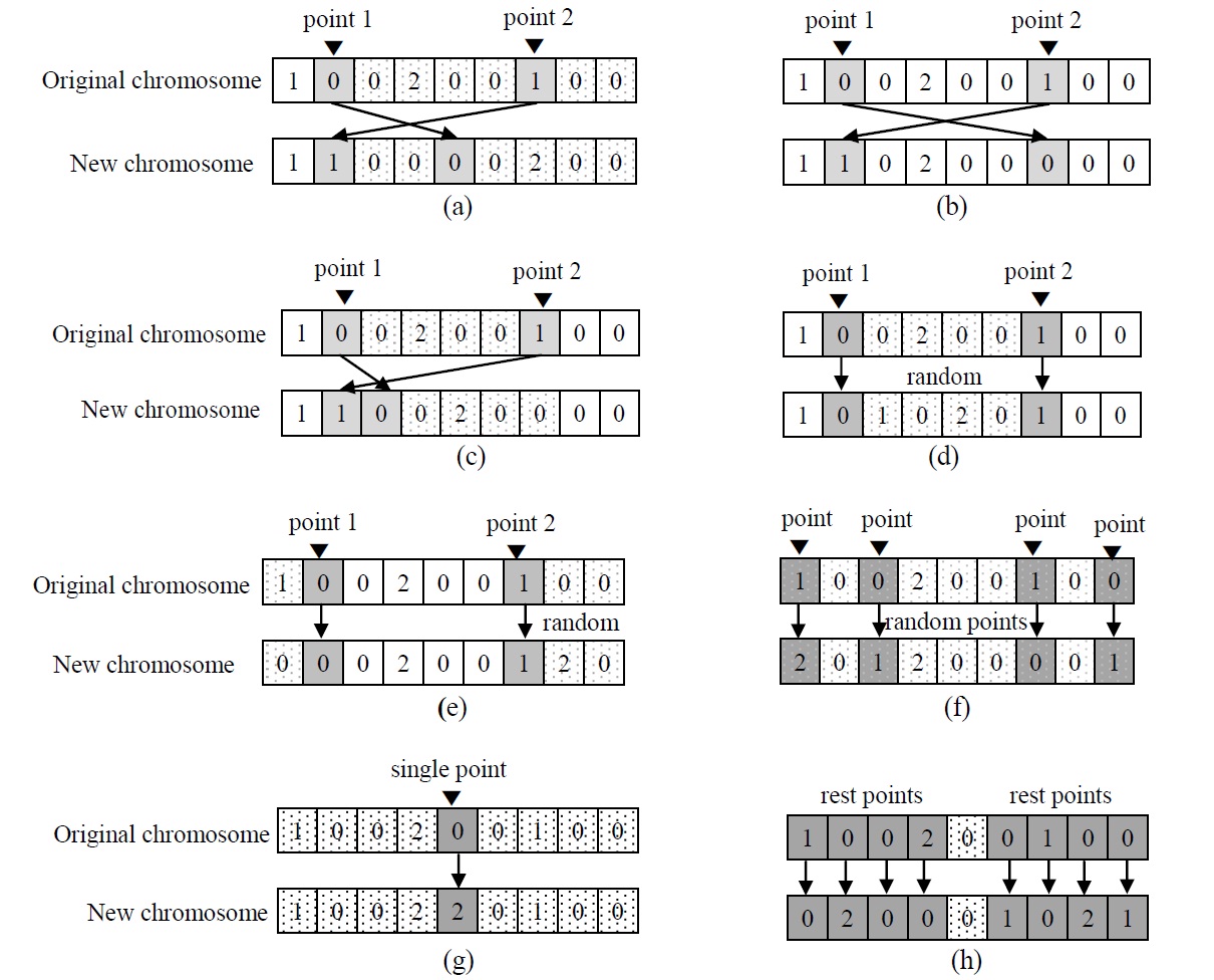
Two kinds of crossover operators are randomly used: partially-matched crossover (PMX) and uniform crossover (UX). Eight kinds of mutation operators are
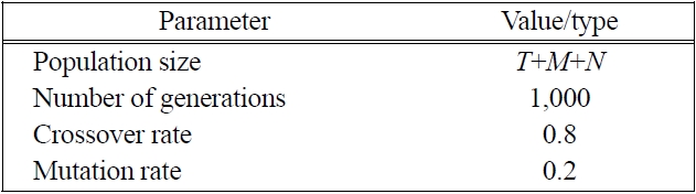
randomly used: the eight kinds of mutation operators (pull operator, swap operator, insert operator, inner random operator, outer random operator, uniform random operator, single change operator, and rest change operator) to make a new chromosome. For the operators, one, two or multiple points in the selected original chromosome are randomly selected and mutated. The pull operator is illustrated in Figure 2a. The genes on right side of point 2 (including point 2) are pulled to the position of point 1, and the genes between point 1 and 2 (including point 1) are placed after. The two genes at the points are interchanged for swap operator as shown in Figure 2b. Insert operator simply insert the gene at point 2 into the position of point 1 as shown in Figure 2c. Inner random operator and outer random operator are illustrated in Figure 2d and e. The inner or outer genes of point 1 and 2 are randomly replaced for the operators. Uniform random operator randomly select multiple points and change as shown in Figure 2f. Figure 2g and h describe single change and other change in simple way. Using the crossover operators, the mutation operators, and the selection operators, the selected parents reproduce new chromosomes (i.e., children) to generate a population for the next generation. The various parameters of the GA heuristic are summarized in Table 1. These parameters were selected based on extensive preliminary experimentations to the best combination with highest performance. GA evaluates a total of 1,000×(
[Table 1.] Parameters of the genetic algorithm heuristics

Parameters of the genetic algorithm heuristics
The following procedure outlines the pseudo code of the GA:
Procedure GA for multi-product lot-sizing problem with a freight container
Begin
Set crossover rate and mutation rate as rc = 0.8 and rm = 0.2
Set a generation size as g = 0
Generate an initial population Pc
Evaluate f ( ? ) all chromosomes in Pc
Find the best chromosome scbest in Pc
Let Pbest = scbest and fbest = f(scbest)
Repeat (the generation loop)
Repeat (the population loop)
Randomly select two parents sc1 and sc2 among the population Pc using roulette wheel selection
Generate two new children sn1 and sn2 by following genetic operations:
If (random [0, 1] < rc )
Then perform randomly PMX crossover or UX crossover
If (random [0, 1] < rm )
Then perform randomly a mutation among 8 mutations
Until (number of populations reaches a maximum of T+M+N)
Evaluate f ( ? ) in Pn
Update Pc by selecting an elitist and the rest of chromosomes in the population using randomly roulette wheel selection or random selection within a good solution pool from Pn
If fbest > f (scbest)
Then
Pbest > scbest and fbest > f (scbest) in the population Pc
Until (number of generation reaches a maximum of 1,000 times)
End
SA was first proposed by Kirkpatrick
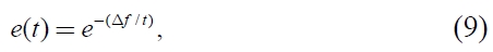
where
In the implementation of this paper, the SA heuristic starts with a randomly generated chromosome and is controlled using two loops: an outer loop and an inner loop. The outer loop controls the temperature reduction according to the cooling schedule. In the inner loop, the temperature is held constant and a predetermined number of explorations are made. In the outer loop, explorations are made at each temperature. For fair comparison with other heuristics, the number of inner loops is 50 and the number of outer loops is 20, and the number of perturbations consists of (
[Table 2.] Parameters of the simulated annealing heuristics
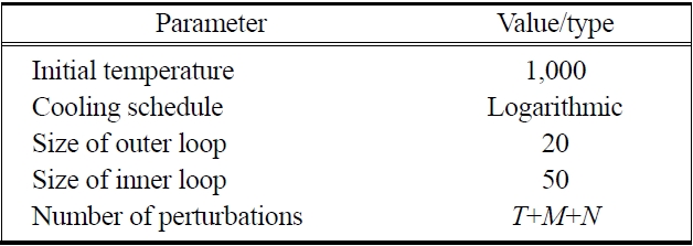
Parameters of the simulated annealing heuristics
The following outlines the outlines pseudo code of the SA algorithm:
Procedure SA for multi-product lot-sizing problem with a freight container
Begin
t = 0
θ0 = 1,000
Randomly select a search point Pc
Evaluate f(Pc)
Let Pbest = Pc and fbest = f(Pc)
Repeat (the outer cooling loop)
Repeat (the inner cooling loop)
Repeat
Apply a specific perturbation on Pc to produce Pn
Evaluate f(Pn) with a local search heuristic
If f(Pn) < f(Pc)
Then
Pc = Pn
If fbest > f(Pn)
Then
Pbest > Pn and fbest > f(Pc)
Else if random [0, 1] < e(f (Pc )? f (Pn )) / θt
Then
Pc = Pn
Until ((T+M+N) random trials are exhausted among 8 perturbations)
Until (number of iterations reaches a maximum of 50 times)
t = t+1
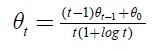
Until (t reaches a maximum of 20 times)
End
SEA is a meta-heuristic algorithm which has a population (a set of solutions) based mechanism that uses the evolution of a solution by itself (self-evolution). Similar to GA, the set of chromosomes forms a population. Initial population is generated randomly, and the chromosomes in the population are evaluated by the measure of the fitness introduced in Section 2. A chromosome from the population is randomly selected and executes a self-reproduction using a random selection of one of mutation operators described in Section 4.2. Then the new chromosome is evaluated and it replaces the original chromosome, if the fitness value of the new chromosome is better than that of the original chromosome. The algorithm continues until the number of self-reproductions becomes a predetermined stopping value.
We propose the operators used in the eight mutations in GA. SEA is running without providing any parameters for the algorithm, because all the selection processes in SEA, such as selection of chromosome from the population for self-evolution, selection of evolution operator, and selection of points for the operator are randomly executed. SEA showed good performance for a machine scheduling problem compared with any other meta-heuristics (Joo and Kim, 2012).
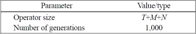
For fair comparison with other heuristics, the number of generations is fixed as 1,000 for terminating, and the number of evolution operators consists of (
[Table 3.] Parameters of the self-evolution algorithm heuristics

Parameters of the self-evolution algorithm heuristics
The following procedure outlines the pseudo code of the SEA:
Procedure SEA for multi-product lot-sizing problem with a freight container
Begin
Set a generation size as g = 0
Generate an initial population Pc
Evaluate f(Pc)
Find the best solution scbest in Pc
Let sbest = scbest and fbest = f(scbest)
Repeat (the generation loop)
Randomly select a solution sc among the population Pc using roulette wheel selection
Apply a specific perturbation sc in the incumbent population Pc to produce sn for the population Pn of the next generation using randomly selected the perturbation operations a mutation among 8 mutations
Evaluate f(sn)
If f(sn) < f(sc)
Then
sc = sn
If fbest = f(sn)
Then
Pbest = sn and fbest = f(sn)
Until (number of generation reaches a maximum of 1,000×(T+M+N) times)
End
To analyze the performance of the proposed heuristic algorithm, the following experimental conditions were designed.
Set M = 3, 6, 10 and T = 4 and 8 in small sized problems and T = 15, 18, and 24 in large sized problems
Demands were generated from a normal distribution,
Mean μi was generated from an uniform distribution, U(25, 100).
Standard deviation σi was equally likely selected from μi or μi/5.
Setup cost was selected by
and TSi = 1, 3, 6, where TSi denotes EOQ time supply.
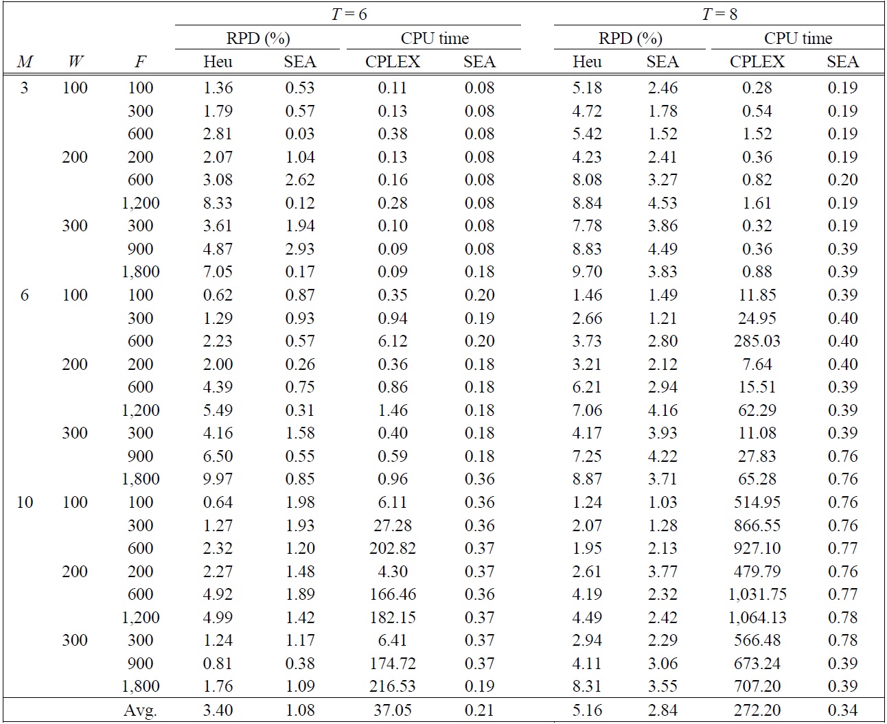
[Table 4.] RPD and CPU times in small sized problems

RPD and CPU times in small sized problems
hti = 1 was assumed without loss of generality.
Set wi were generated from an uniform distribution, U(0, 5)
W = 100, 200, 300 and respective unit freight cost was proportionally selected by W as follows:
F =i ? W, i =1, 3, 6.
To evaluate the performance of the heuristic, the C# computer code for the proposed heuristic was run on an Intel Core™2 Duo CPU with 2.00 GHz RAM. Also, CPLEX package for finding the optimal solution was run on the same computer and run so as to find the best solution within 700,000 node limits.
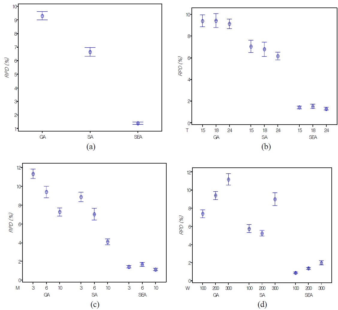
For the performance of the heuristics, the relative percentage deviation (RPD) calculated with the expression (10) and the computing time by GA, SA, and SEA of 10 replications for each test problem.
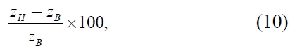
Where
In small sized problems, four instances were made for each combination of input parameters and 10 replicates for each instance are performed in the meta-heuristics (GA, SA, and SEA). In Table 4, we compare SEA shown in the best performance among SA and GA with the local search heuristic (Heu) proposed by Kim and Lee (2012). In the second column in the Table 4, SEA shown in the best performance offers on the no more than 5% from the optimal solution with small computa-
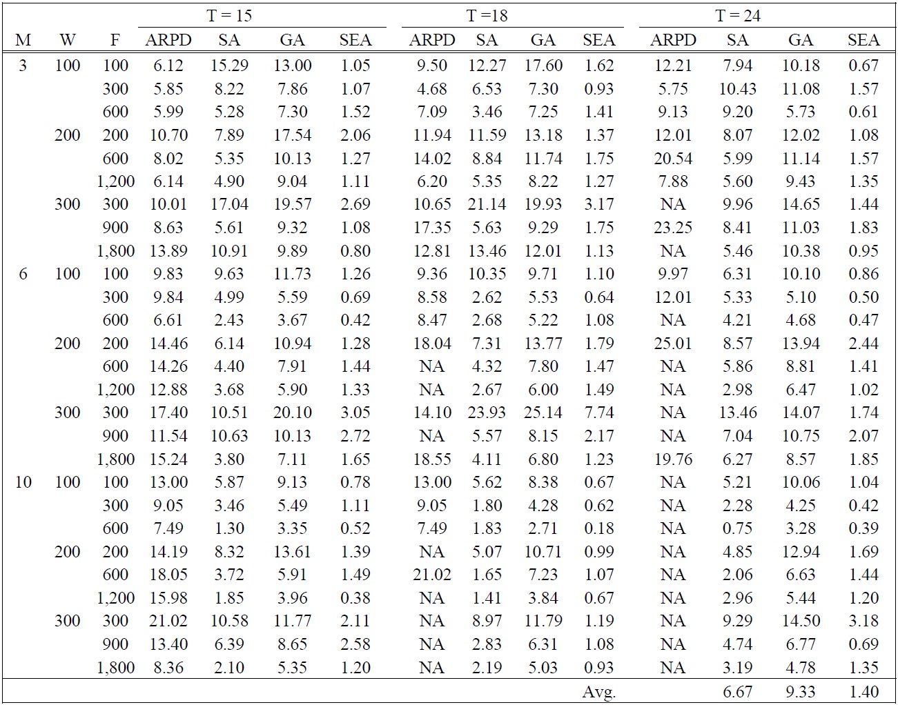
Absolute RPDs between CPLEX and SEA and relative RPDs among SA, GA, and SEA in large sized problems
tional time for small sized test problems. The difference of RPDs between SEA and Heu increases as
In large sized problems, the absolute performance between CPLEX and the best solution of the heuristics (ARPD) is presented with the expression (11) and the relative performance of the heuristics (SA, GA, and SEA) is compared by the best value of the heuristics are shown in Table 5.
Where
Table 5 shows that the optimal solution using CPLEX was not obtained within 1 hour for many large-sized test problems having more than 15 periods as shown in ‘NA’ because of the limitations of a computer performance. This result indicates that it is difficult to find the optimal solution as the problem size increases (
In this paper, a dynamic lot sizing problem and shipment scheduling are simultaneously analyzed, where the order size of multiple products and a single container type are simultaneously considered. To address the problem, two different solution approaches are proposed. The first approach is based on a mixed integer programming model. Because the problem is NP-hard, three meta-heuristic algorithms are proposed to increase solution efficiency based on the optimal solution properties. SEA is a new meta-heuristic algorithm which has a population (a set of solutions) based self-evolution mechanism. Two problem groups are tested to verify the performance of proposed meta-heuristic algorithms. SEA offers the best performance by showing 1.40% of RPD value in average sense compared to SA and GA. Also, the RPD value of SEA is consistent with small variance as
Further study is required to assess the performance of SEA with other meta-heuristics (tabu-search and antcolony optimization, etc.) in solving the inbound ordering problem.