Generally, it is possible to obtain conformal mapping by numerical methods. The methods of numerical conformal mapping are usually classified into those that construct the map from a standard domain such as the unit disk onto the 'problem domain', and those which construct the map in the reverse direction. The former is derived from a non-linear equation, and the other is obtained from a linear equation.
We treat numerical conformal mapping from the unit disk onto the Jordan regions as the problem domain here. The traditional standard methods of this type are based on the Theodorsen integral equation [1].
It is the goal of numerical conformal mapping to find methods that are at once fast, accurate, and reliable.
This paper discusses the numerical conformal mapping from the unit disk onto the Jordan region, which can be solved by the Theodorson equation, a nonlinear integral equation for boundary functions.
There are a number of methods for solving the Theodorsen equation. Here, we deal with the Niethammer method based on successive over-relaxation (SOR) iteration and the Wegmann method based on Newton iteration.
The Wegmann method has been known to be the most effectively economical one in calculation and memory. This iterative method is based on a certain Riemann-Hilbert problem to sharply reduce the space of calculation and memory [1].
After we had several numerical experiments for these two methods, we found that the Niethammer method is more effective than the Wegmann method in the easy problem case and the Wegmann method is more effective than the Niethammer method in the difficult problem case.
We begin with defining the functional space by some signs used in this paper.
t ∈ T is used as a variable for a 2π periodic function, where T is the quotient space T ? R/2πZ (R is a real number and Z is an integer).
We define the notations below as follows:
C(T) : 2π periodic complex continuous function space
CR (T): 2π periodic real continuous function space
Cm(T) (m ≥ 1) 2π periodic complex function space of m times differentiable

(T) (m ≥ 1): 2π periodic real continuous function space on m times differentiable

complex continuous function space being analytic in D and continuous in

, where D is the interior of a unit circle
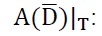
set of boundary functions f, f(t) =h(eit) for

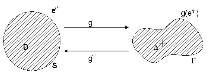
Let g be a conformal map of the unit disk D with boundary S onto a given Jordan domain Δ with boundary Γ. We assume g is normalized by g(0)=0 and g’(0)> 0 . Then the map g can be extended to the closure
of D, inducing a conformal map g: S → Γ (Fig. 1).
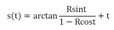
Therefore the problem of computing g: S → Γ becomes to the problem of computing s(=s(t)) satisfying

where [Im η(s)]0 is 0 dimensional Fourier coefficient.
Definition 1.
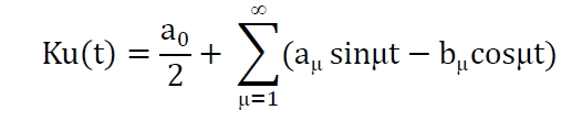
If a continuous function u(t) is expended by Fourier series as follows:
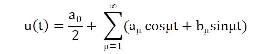
we define K as the conjugate operator in the below definition,
Here is another theorem concerning the boundary function and conjugate operator [2].
Theorem 1.
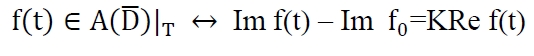
, where f(t) is a boundary function, Imf(t) is f(t)’s imaginary part, Ref(t) is f(t)’s real part, and f0 is f’s 0 dimensional Fourier coefficient.
The normalized condition (1) makes Im η0=0 possible. Using Theorem 1, we derive a boundary function η(s) as follows:

Formula (2) leads to the below Eq. (3) by which we can get s:

We call this formula (3) the Theodorsen equation.
Among the various solutions for this nonlinear equation, we discuss Niethammer’s method using SOR and Wegmann’s method using Newton.
For numerical calculation, we make a discretization, using even discrete number N = 2n for use Fourier transform.
Choose equidistant points tv = 2πv/N, v=0,1,2,…N-1 in the interval [0, 2π].
fj is defined as follows:
fj ? f(tj ), f: = (f0, f1 … , fN-1)T.
In addition, a scalar function σ(y) and vector
y: = ( y0 , y1, … , yN-1)T are defined as
σ(y) ? (σ(y0), σ(y1), … , σ(yN-1))T .
The conjugate operator is discretized as follows:
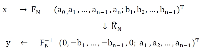
Where FN is a discrete Fourier transform,

is an inverse discrete Fourier transform, and

is a Fourier coefficient transformation by conjugate operator [3].
Thus a discrete conjugate operator can be as
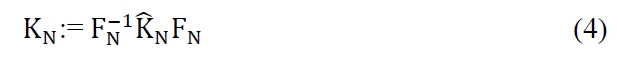
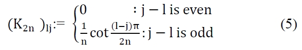
We call (4) the Wittich matrix and each components are
Assume the boundary function of the Jordan region (problem domain) is given by η(t) = ρ(t)eit.
Then the Theodorsen equation (3) leads to the equation below in its discrete version
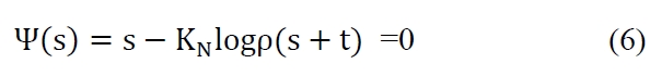
Among the various solutions for this nonlinear Eq. (6), we discuss Wegmann's method with Newton and Niethammer’s method with SOR.
Niethammer solved Thedorsen equation (6) with SOR (successive over-relaxation) [2].
We define ? and ? as follows:

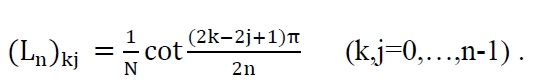
We define
and apply this to (5), then
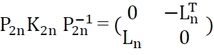
, where
Therefore, the solution of (6) is obtained as follows:
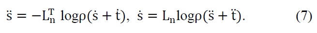
Then (7) becomes
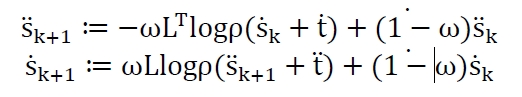
(0 <
L, LT are calculated effectively by fast Fourier transform (FFT).
Wegmann solved the original nonlinear Eq. (6) with Newton’s method as
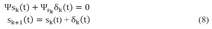
Ψsk: differential of Ψ with respect to sk, k=1,2,…,
δk: correction in the k th step .
Wegmann reduced calculation and memory space by rendering it a Riemann-Hilbert problem on the unit circle [4]. The iteration scheme can be performed numerically in the following way. If initial value s0 is determined we can calculate an approximate value sk (k=1,2, … ) with following formulas (9-1) to (9-6) [4, 5].


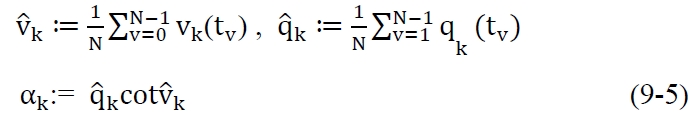
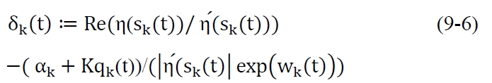

where η′(sk) is the differential of η with respect to sk .
Wegmann's method has been known to be the most effectively economical one in capacity for calculation and memory [2]. This iterative method is based on a certain Riemann-Hilbert problem to sharply reduce the space of calculation and memory. In addition, the speed of a convergence is fast with few errors [4].
However, we have several numerical experiments; they appear to be diverge greatly from the iterative method of Wegmann. We may say that the iterative method comes to be unstable in that the divergence occurs especially when some degree of difficulty is high [6].
We treat eccentric circle, which is a problem domain, as the example of a numerical experiment. We are able to estimate the correct errors because the real value of this example is known.
The eccentric circle has the following function on the boundary:
η(s) = ρ(s)eis
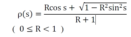
Real value:
This is an example of a problem which is getting difficult as R becomes larger toward 1 because the transformation is more and more serious. Set the initial value to s0 = (0,0, … ,0)T and required error to ∥ sk ? sk+1 ∥2<10?5, k=1,2,…, .
The meaning of signs which show the results of the experiments is as follows:
N: Discrete number
R: Configuration parameter
ω: Relaxation coefficient
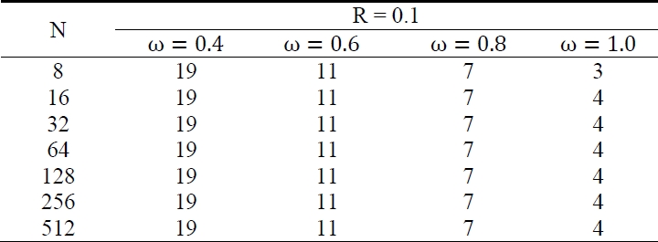
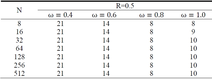
Table. 1-3 show the results that we had experiments with Niethammer’s method, which are the iteration numbers at R = 0.1, 0.5 and R = 0.9 when iteration was convergent at ω = 0.4-1.0 with 0.2 interval.
There, we can see that the iteration numbers are changed by the configuration parameter R not by the discrete sample points N when ω is fixed.
The most suitable relaxation coefficients ω are 1.0 at R= 0.1, 0.8 at R = 0.5 and 0.6 at R = 0.9. That means the relaxation coefficient ω is smaller as configuration parameter R becomes larger toward 1; that is, the transformation is more serious.
[Table 1.] The iteration numbers at R = 0.1

The iteration numbers at R = 0.1
[Table 2.] The iteration numbers at R = 0.5

The iteration numbers at R = 0.5
[Table 3.] The iteration numbers at R=0.9
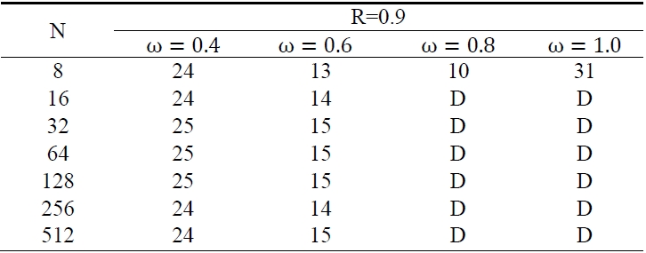
The iteration numbers at R=0.9
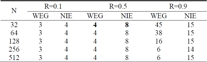
Table 4 shows the results which had experiments with Wegmann’s method using Newton iteration and Neithammet’s method using SOR. These are the iteration numbers when the both iteration were convergent. The results of Niethammer’s method are the iteration numbers with most suitable relaxation coefficient ω.
There, we can see the Wegmann’s method has iteration numbers 3 at R = 0.1 and 4 at R = 0.5, that is, this method has quadratic convergence at R = 0.1 and 0.5 but its convergence speed comes to be slow at R = 0.9.
However the convergence speed comes to be faster when the discrete number is increased.
We can estimate the reason that the iteration comes to be slow when the discrete number is small is discrete errors. In Table 4, we can see the convergence speed of Wegmann’s method is faster than that of Niethammer’s method. Wegmann’s is more efficient than that of Niethammer’s on the difficult problems in which the degree of the problem is high. On the other hand, in Table 5 we can see that Nithammer’s method is more efficient than Wegmann’s method on the easy problems in which the degree of the problems is low. The time complexity of Niethammer is smaller than that of Wegmann as Table 5 shows.
[Table 4.] The iteration numbersby Wegmann (WEG) and Niethammer (NIE)
The iteration numbersby Wegmann (WEG) and Niethammer (NIE)
[Table 5.] Comparison of numerical solutions
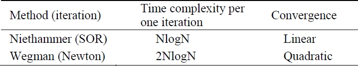
Comparison of numerical solutions
Conformal mapping has been a familiar tool of science and engineering for generations.
This paper discussed the numerical conformal mapping from the unit disk onto the Jordan region, which can be solved by the Theodorson equation, a nonlinear integral equation for boundary functions.
There are many methods for solving the Theodorsen equation. Here, we deal with Niethammer’s method based on SOR iteration and Wegmann’s method based on Newton iteration.
Wegmann’s method is well known as very efficient one in speed and memory. An improved method for convergence by applying a low frequency pass filter to this method has been proposed [7, 8].
We analyzed and experimented with Nithammer’s method using SOR and compared Wegmann’s method using Newton as the solutions of the Theodorsen equation for numerical conformal mapping in this paper.
Through our numerical experiments, we can see that Wegmann’s method is more efficient when the problem is difficult and the required accuracy is high, while Niethammer’s method is more efficient on the easy problems.
The determination of the most suitable relaxation coefficient ω is very important in Niethammer’s method. In our experiments by Niethammer’s method, we found that as the problem becomes more difficult.
Futher theoretical research should investigate the most suitable relaxation coefficient ω.