Active studies on holography, which is the ideal and final goal of 3-dimensional (3D) image display, have been undertaken mainly in the US, Europe, and Japan. In particular, real-time holographic video is the core technology for the next-generation 3D television (TV).

The computer-generated hologram (CGH) was proposed by Brown and Lohmann [1] in 1966. It obtains an interference pattern through an arithmetic operation on a personal computer (PC) by approximating optical signals. Thus, it is easy to obtain a digital hologram (DH) with this CGH method for real and virtual objects. The problem with this method is that it exhausts much calculation time. For example, to calculate a DH using the CGH method, approximately 900 seconds are required if a general PC is used to display a significant quantity of computation (3D object measuring approximately 1 × 1 × 1 cm in space). To resolve this problem, Yoshikawa [2] tried to increase the calculation speed by recursively adding only the distance difference between a source point on the 3D object and the digital hologram to be generated. In [3], another recursive technique was proposed where only the leftmost pixel of a row in a digital hologram is fully calculated and the remaining pixels of the row are recursively calculated such as by adding the pre-calculated values and the previously calculated results to the results for the first column pixel of the row.

The purpose of this paper is to analyze a CGH method for calculation speed to generate a digital hologram. We analyze previous recursive methods [3] to identify the regularity between the depth-map image and the digital hologram.

In section II, previous CGH methods are described. Section III contains analysis of the CGH method and then optimization of the CGH method. Our conclusions are given in section IV.

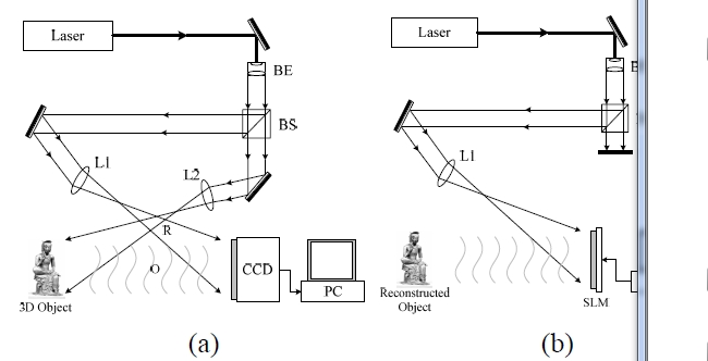
A system for digital holograms uses electronic equipment such as charge coupled device (CCD) cameras instead of optical ones to record the interference pattern of the holography and transmit it as a video signal. The image is reconstructed on the receiver side by illuminating a laser beam onto the received interference pattern uploaded on a spatial light modulator (SLM). Fig. 1 shows configurations of this system at the transmitter side (a) and the receiver side (b), which are the same configurations as the optical ones other than the CCD camera. That is, the recording system sends laser beams into the collimated wave using the condensing lens, and divides the wave into a reference wave and an object wave using a beam splitter. The object wave is illuminated onto the object while the reference wave is directly illuminated to the CCD camera. Then the two waves form an interference pattern and the CCD camera seizes this pattern. To reconstruct the hologram image, the interference pattern information is uploaded in the SLM to which a collimated wave is illuminated. Then the first diffraction beam is generated and the real image is reconstructed at the same position [4].

This section describes the previous CGH calculation method and the one using the recursive addition system.

The CGH generating equation is defined as Eq. (1),

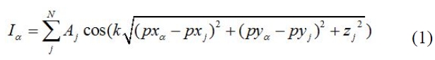
where α or j indicates a particular point on the hologram or 3D object, respectively, k is the wave number of the reference wave defined as 2π/λ, p represents the pixel pitch of the hologram, and (x_α , y_α) and (x_j, y_j, z_j) represent the coordinates of the hologram and 3D object, respectively.

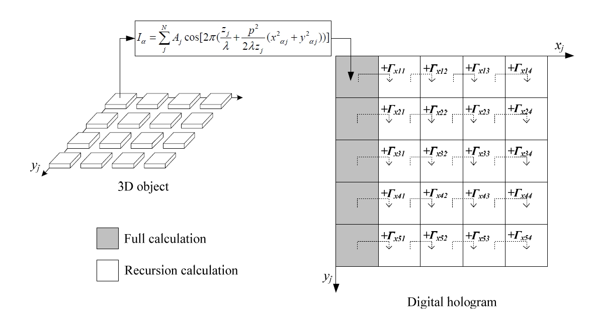
Fig. 2 shows a sample coordinate array system for the 3D object and the digital hologram to apply the CGH method, where the 3D object in 2 × 2, and the DH is captured as 4×4 in size. To generate a DH with this set-up, the calculation of Eq. (1) must be carried out 64 (= 2 × 2 × 4 × 4) times.

If Eq. (1) is approximated to the first term after the Taylor expansion, it would be as Eq. (2).

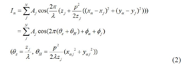
Here, x_αj and y_αj mean (x_α-x_j) and (y_α- y_j). The phase θ_H(x_αj+n, y_αj, z_j) at one point (x_α+n, y_α) of the digital hologram can be expressed as,

Here, Γ_xn is defined as,

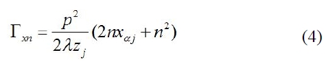
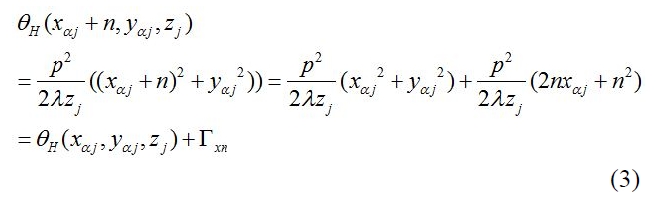
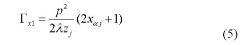
In the case of n = 1, that is Γ_x1, Eq. (4) would be,

Meanwhile, in the case of n = 2, Γ_x2 is,

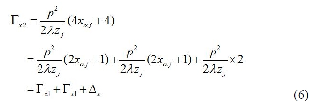
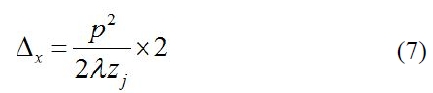
where Δ_x is defined as,

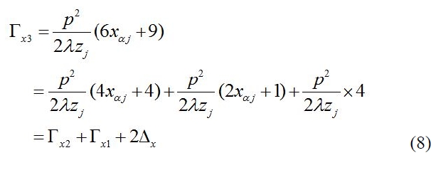
Again, when Γ_x3 is calculated with n = 3,

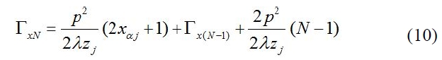
When n = N, Γ_xN can be generalized as,

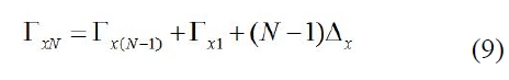
From Eq. (9) it is clear that, once the first column (the leftmost pixel) of a row of a digital hologram (Γ_x1) and Δ_x for a light source are calculated, the remnant pixel values (Γ_xN) of the row with the same light source can be recursively calculated by adding Γ_x1, Δ_x, and the previously calculated value (Γ_x(N-1)).

At this time, we name the CGH calculation in Eq. (2) full calculation and the calculation by Eq. (9) recursion calculation. Fig. 3 shows the method of [3] described above. The gray blocks in the figure are the results from the full calculations and the white blocks are the results of the recursion calculations. To obtain a 1,024 × 1,024 DH for an object with the light sources of 200 × 200, the ordinary method with only full calculation needs 1,024 × 1,024 × 200 × 200 = 41,943,040,000 full calculations. But with the previous method, only 1,024 × 200 × 200 = 40,960,000 full calculations are necessary and the remnant 1,023 × 1,024 × 200 × 200 = 41,902,080,000 calculations would be recursion calculations. In other words, this method reduces more than 99.9% of the full calculations and the remnant calculations can be replaced with much simpler recursion calculations.

As discussed in section II-A, the previous CGH method is a more advanced calculation method compared with the conventional method that carries out the full calculation to a level on a par with the quantity of all points of the 3D object, and the quantity of the coordinates of the hologram.

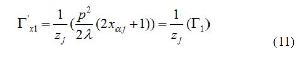
If the original equation is substituted for Γ_x1 and Δ_x of the Eq. (10), it becomes the same as the following:

Eq. (11) implies that when one point of the 3D object is calculated from the first x-axis (x-axis beginning with the (0,0) coordinate) of the hologram, the variable that changes the value after Γ_x2 is only N. That is, if one point of the 3D object is computed, the Γ_xN computed from the first x-axis of the hologram becomes the same as the Γ_xN values of the other x-axis. Accordingly, the Γ_xN calculated at the same time with the first x-axis holograms that have been computed can also be used with another x-axis hologram that has been calculated.

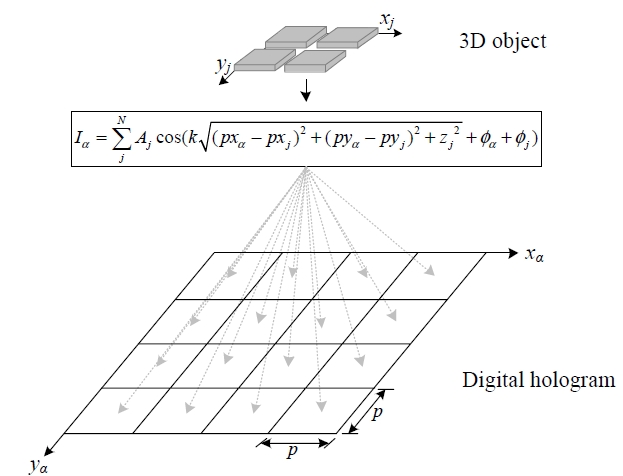
The application of the previous method can be expanded to a case where the CGH calculation is carried out on the points that exist on the same column of the 3D object as shown in Fig 4. However, the pre-calculated Γ_xN values cannot be used repeatedly because, even though the x_j, x_a, N values are the same when the points on the same column are recursively added using Eq. (11), z_j is changed. To solve this, we can process Eq. (11) as below.

In the case of N = 1, Γ’_x1 is

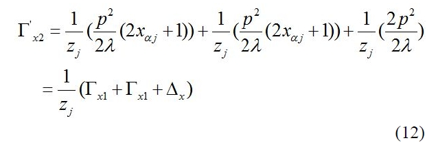
In the case of N = 2, Γ’_x2 is

In the case of N = 3, Γ’_x3 is

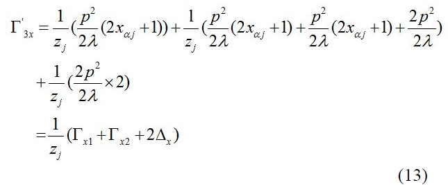
And Γ’_xN in the case of n = N can be generalized as follows.

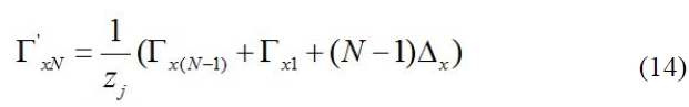
As shown in Eqs. (9) and (14), the Γ’_xN values used are identical when carrying out the CGH calculation on the 3D objects of the same column, except z. This means that when the recursive addition CGH calculation of the x-axis is carried out on the points that existed in the same column of the 3D object, the remaining terms, excluding z_j can reduce the calculation time by using the Γ’_xN values of the first point as it is.

Applying the x-axis recursive operation method of the previous method explained in section II-B to the y-axis direction of the DH can be summarized as follows.

The phase θ_H (x_αj, y_αj+n, z_j) can be expressed as follows from one point (x_α, y_α+n) of the DH.

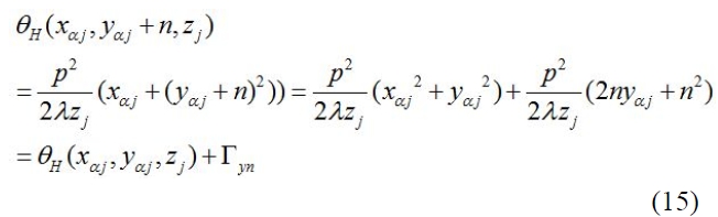
Here, Γ_yn is defined as follows.

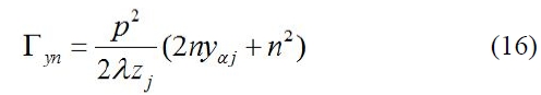
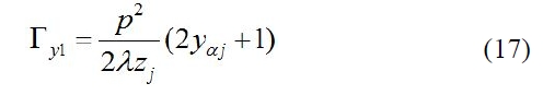
In the case of n = 1, Γ_y1 is

and, in the case of n = 2, Γ_y2 is

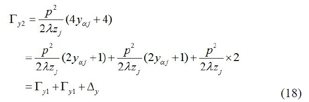
Here, Δ_x is defined as follows:

Again, when Γ_y3 is calculated in the case of n = 3,

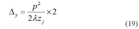
Γ_yN can be generalized as follows in the case of n = N.

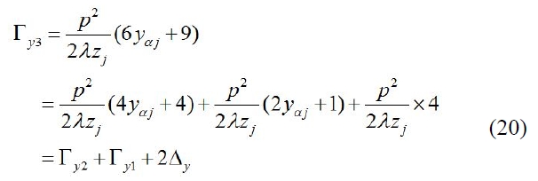
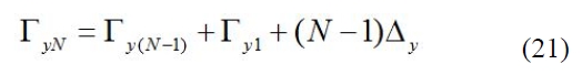
When Eqs. (9) and (21) are compared, they are apparently identical. That is, the recursive CGH calculation method in the direction of the x-axis proposed in [3] can be expanded and applied to the y-axis direction.

To find regularities between the points located on the same column of the 3D object, the actual values were applied to Eq. (21) to calculate Γ_yN, and the results are shown in previous equations. Such regularity can be generalized as Eq. (22).

Eq. (22) indicates that when the recursive CGH calculation in the direction of the y-axis is carried out on the points located in the same column of the 3D object, the values calculated based on Eq. (22) are recursively added to the value calculated from the first coordinate ((0,0)) of the hologram. That is, the Γ_yN that is calculated at the same time with the calculation of the points in the same first column of the 3D object can be used as it is for the operation on the second points below, reducing the operation time.

In this paper, we analyzed a CGH method for calculation speed to generate a digital hologram. We analyzed the previous recursive method [3] to identify the regularity between the depth-map image and the digital hologram.

It is expected that the analyzed CGH algorithm covering the whole coordinate array of the hologram proposed in this paper will be a core fundamental technology of the holographic 3DTV system for next-generation TV.