Technological advances in sensors and wireless communications have enabled offering of high location accuracy in location tracking at a low cost [1-3]. Such accuracy gave rise to a series of location-based applications that exploit positional data to offer high-end location-based services (LBS) to their subscribers[4]. Conversely, mobile users require the protection of their context information (e.g., location and/or identity information)against privacy adversaries (e.g., Big-brother type threats,users profiling, unsolicited advertising) [5-8]. The privacy issue is amplified by the requirement in modern telematics and location-aware applications for real-time, continuous location updates and accurate location information (e.g., traffic monitoring, asset tracking, location-based advertising, location-based payments,routing directions) [9-11].
We consider a population of mobile users who are supported by some telecommunication infrastructure, owned by a telecom operator. Every user periodically transmits through his/her mobile device a location update to some traffic monitoring system residing in a untrusted Internet-connected LBS provider. A trusted server in the telecom operator plays the role of a proxy that mediates between the user and the LBS provider. Our setting involves an LBS provider that is requested to efficiently answer Range Queries (RQs) of mobile users moving on the plane. For example historical queries of the form:
SELECT Count (Mobile-User-Ids)
FROM Moving_Object_Database (MOD)
WHERE spatial-area=MBR(‘Acropolis’) and
or prediction queries of the form:
SELECT Count (Mobile-User-Ids)
FROM Moving_Object_Database (MOD)
WHERE spatial-area=MBR(‘Acropolis’) and
that provide traffic monitoring services to mobile users. This type of query focuses on the problem of indexing mobile users in two dimensions and efficiently answering range queries over the users’ locations. This problem is motivated by a set of reallife applications, such as intelligent transportation systems, cellular communications, and meteorology monitoring.
Our privacy requirements, include:
? Location privacy:The protocol does not reveal the (exact)user’s location information to the LBS provider.
? Tracking protection (Unlinkability):The LBS provider is not able to link two or more successive user positions.
In our privacy threat model, we assume an attacker has access to the k-anonymized (cloaked) location queries and to the algorithms used by the trusted server to support user privacy.We assume that the proxy server of the telecom operator is trusted not to collude with the LBS provider or other internal/external non-authorized entities to expose the atomic location updates of system users.
Traditionally, the transformation of the exact user location to a spatiotemporal area is achieved by the k-anonymity principle for relational data [12, 13]. This requires that each record in a given dataset is indistinguishable from at least
>
A. High Level Description of Our Framework
As part of our framework, we deliver the type of
The proposed framework deals with the event of failure in the provision of
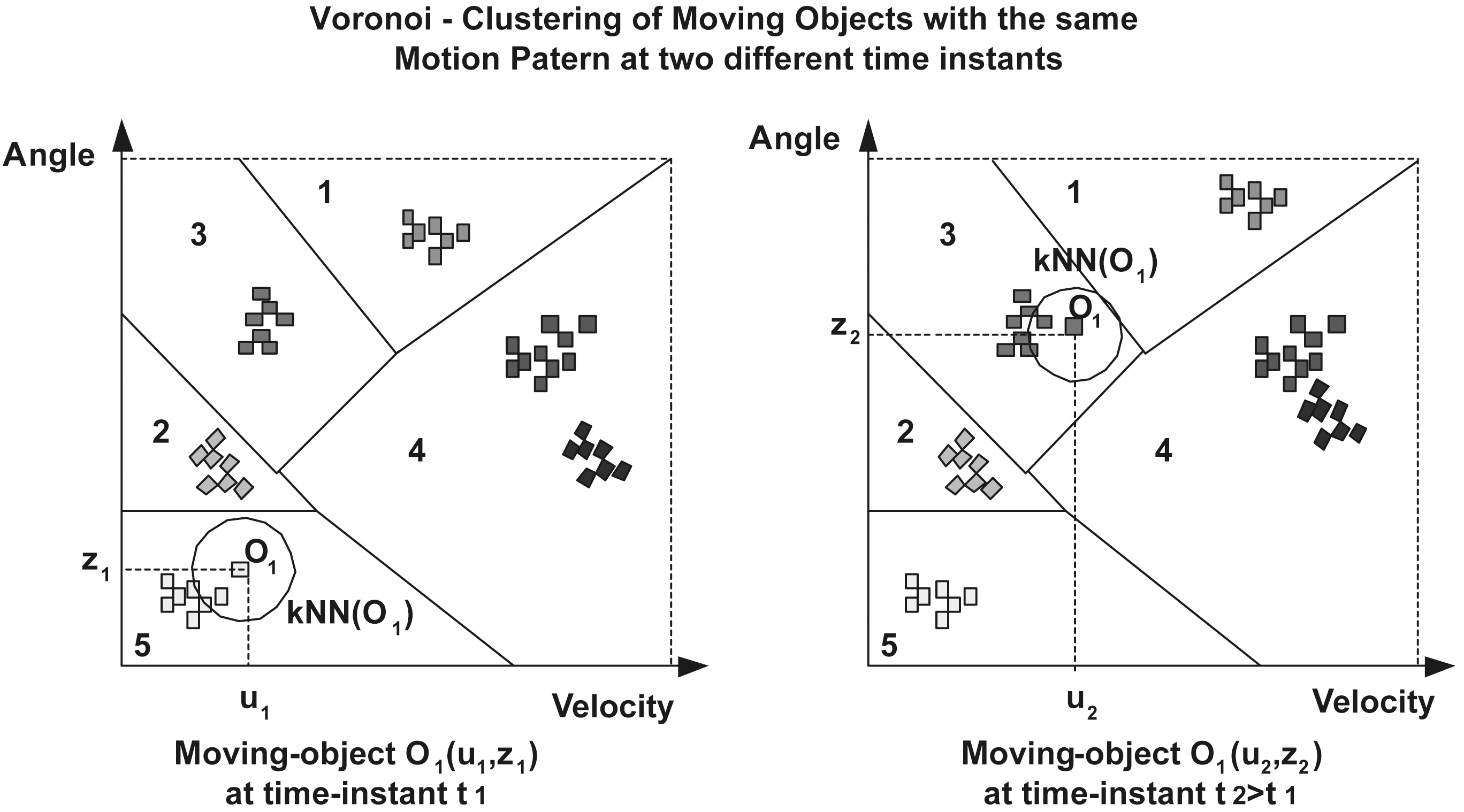
The proposed privacy framework can be reinforced by clustering the mobile users according to their motion patterns on the(
Two basic approaches are used when trying to handle RQ services; those that deal with discrete and those that deal with continuous movements. In a discrete environment the problem of dealing with a set of moving objects can be considered to be equivalent to a sequence of database snapshots of the object positions/extents taken at time instants t1 < t2 < . . ., with each time instant denoting the moment where a change took place.From this viewpoint, the indexing problems in such environments can be dealt with by suitably extending indexing techniques from the area of temporal [15] or/and spatial databases[16]; in [17] it is elegantly exposed how these indexing techniques can be generalized to handle efficiently queries in a discrete spatiotemporal environment. A plethora of efficient data structures exists that consider continuous movements [18-22].The common thrust behind these indexing structures lies in the idea of abstracting each object’s position as a continuous function f(t) of time and updating the database whenever the function parameters change; accordingly, an object is modeled as a pair consisting of its extent at a reference time (design parameter)and its motion vector. One categorization of the aforementioned structures is according to the family of the underlying access method used. In particular, there are approaches based either on R-trees or on Quad-trees. Conversely, these structures can be also partitioned into 1) those that are based on geometric duality and represent the stored objects in the dual space [19,21] and 2) those that leave the original representation intact by indexing data in their native n-d space [20, 22, 23]. The geometric duality transformation is a tool heavily used in the Computational Geometry literature that maps hyper-planes in Rn to points and vice-versa. We implement a framework based on the proposed privacy model that uses the Spatial extensions of MySql 5.x to offer privacy in RQ services.
In this work, we study the problem of privacy-preservation data publishing in moving objects databases. In particular, the trajectory of a mobile user in the plane is no longer a polyline in a two-dimensional space, instead it is a two-dimensional surface:we know that the trajectory of the mobile user is within
this surface, but we do not know exactly where. We transform the surface’s boundary polylines to dual points [19, 20] and we focus on the information distortion introduced by this space translation. We develop a set of efficient spatiotemporal access methods and, we experimentally measure the impact of information distortion by comparing the performance results of the same spatiotemporal range queries executed on the original database and on the anonymized one.
The remainder of this paper is organized as follows. Section II lays out the system model for our proposed methodology and gives a formal description of the problem. Section III discusses preliminary notions and results used throughout the paper. Section IV presents the method of transforming the trajectory polylines to two-dimensional surfaces. Section V presents: 1) the duality transformation of the surface’s boundary poly-lines, 2) a simple observation, based on which we enforce the privacy model of our method, and 3) the information distortion introduced by this space translation. Section VI presents an extended experimental evaluation. Section VII concludes the paper.
II. SYSTEM MODEL AND PROBLEM DESCRIPTION
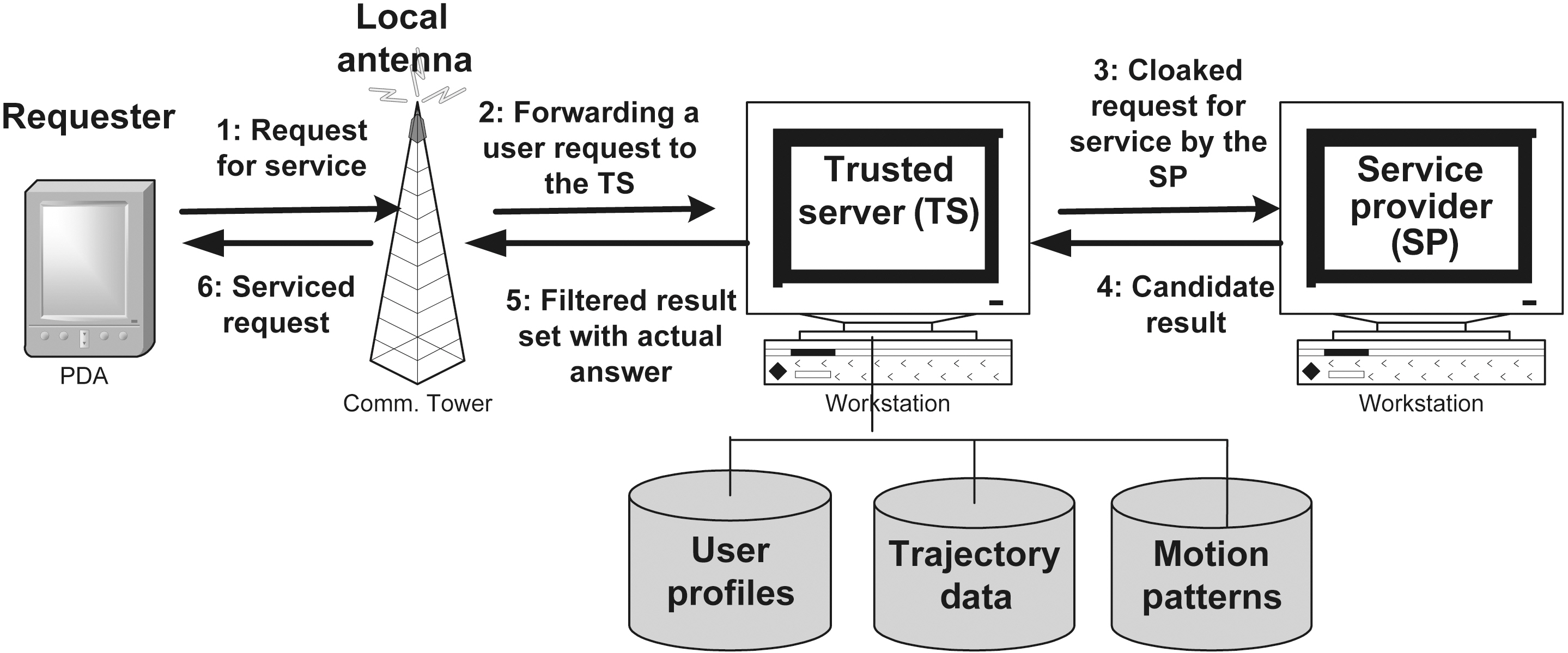
This section lays out the system model in which our proposed methodology is applied. The considered system framework interconnects a set of registered LBS providers to a set of subscribed users, to enable the offering of RQSs in a privacyaware manner. Fig. 1 depicts our system framework that has two main components: the trusted server, which is assigned the task of trajectory privacy preservation, and the service providers,which offer the actual RQSs. As part of its functionality, the trusted server maintains a database that stores the privacy profiles of the users, their history of movement, as well as knowledge of motion patterns.
A system user can be any individual who is equipped with a mobile device and is registered to the trusted server. Upon his/her registration, the user is assigned a unique profile in the system and his/her movement is subsequently monitored by the trusted server. The tracking of user movement is enabled by the transmission of periodic location updates from the mobile device of the user to the trusted server. A privacy profile for a user consists of a set of tuples (sid, K, Amin) that define his/her privacy requirements that involve 1) the value of k for each provided service sid, where k indicates that the user wants to remain K-anonymous when using this service, and 2) the minimum area of generalization Amin, where Amin indicates the minimum spatial area to which the anonymized request should point.
Fig. 1 depicts the regular scenario for the privacy-aware provision of RQSs. Whenever a user requests an RQS (step 1), the trusted server receives the original request (step 2), examines the point of request and determines the appropriate anonymity strategy that needs to be enforced. Next, the original request is transformed to a ’secure’ equivalent that preserves the k-anonymity of the requester and is forwarded to the appropriate service provider to be serviced (step 3). After the request has been serviced, the result set, computed by the service provider, is returned to the trusted server (step 4) where it is filtered to contain only the actual answer that is subsequently forwarded to the requester (steps 5 and 6). This concludes the privacy-aware provision of the service.
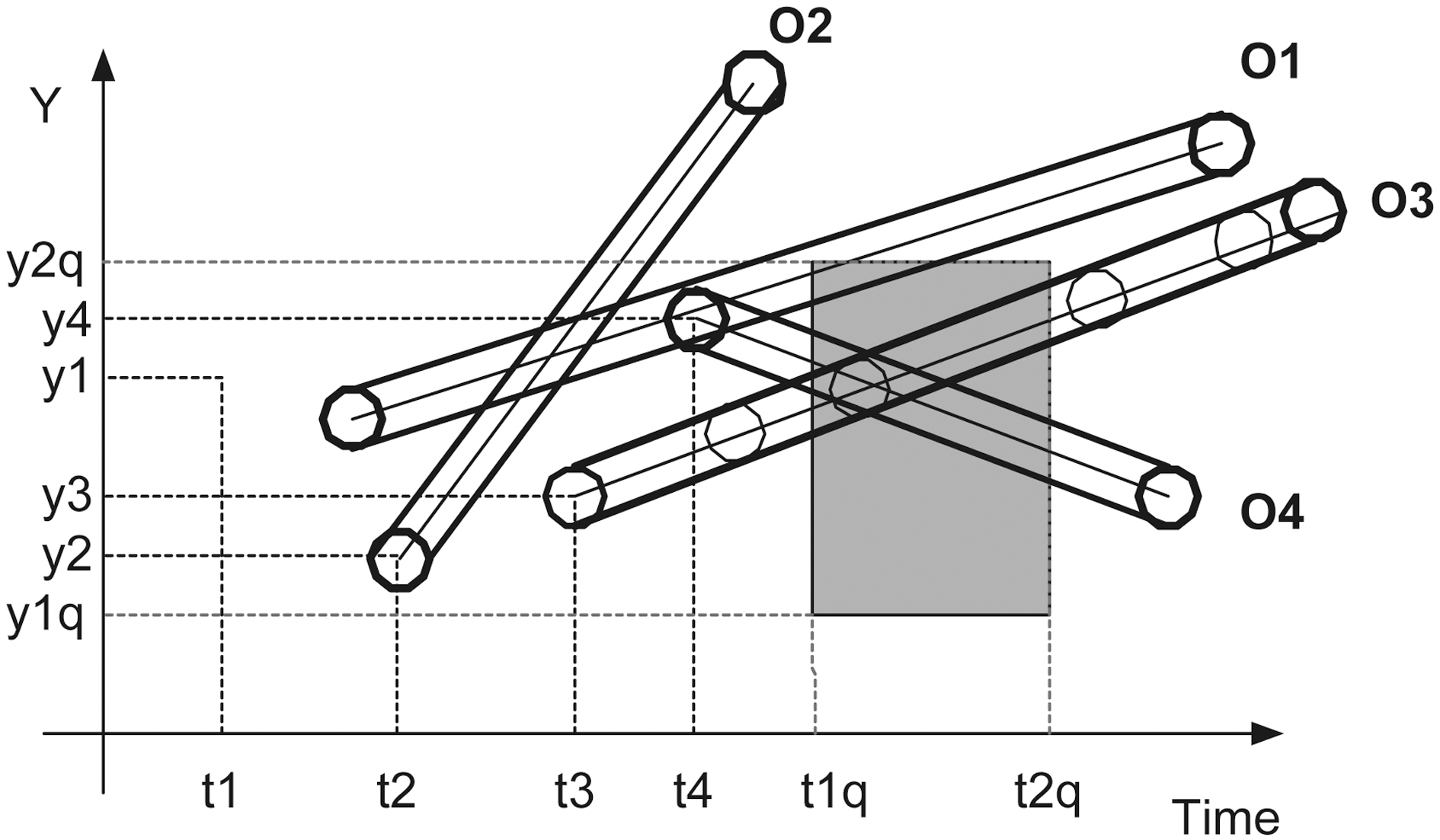
We consider a database that records the position of moving objects in two dimensions on a finite terrain. We assume that objects move with a constant velocity vector starting from a specific location at a specific time instant. Thus, we can calculate the future object position, if its motion characteristics remain the same. Velocities are bounded by [umin, umax]. Objects update their motion information, when their speed or direction changes. The system is dynamic, i.e., objects may be deleted or new objects may be inserted. Let Pz(t0) = [x0, y0] be the initial position at time t0 of object z. If object z starts moving at time t> t0, its position will be Pz(t) = [x(t), y(t)] = [x0 + ux(t ? t0), y0 +
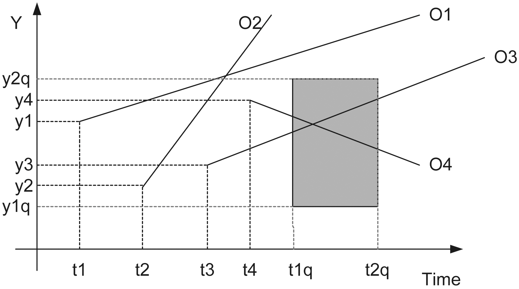
uy(t ? t0)], where U = (ux, uy) is its velocity vector. For example,in Fig. 2 the lines depict the objects trajectories on the (t, y)plane. We would like to answer queries of the form:“Report the objects located inside the rectangle [x1 q, x2 q] ×[y1 q, y2 q] at the time instants between t1 q and t2 q (where tnow ≤ t1 q ≤t2 q), given the current motion information of all objects.”
In the following, we briefly describe the most basic methods for indexing mobile objects, as well as the best current clustering algorithms that will be used throughout the paper and specifically for clustering mobile objects with similar motionpattern.
>
A. Literature Survey: The Most Basic Methods for Indexing Mobile Objects
In the sequel, let N denote the input size (number of stored objects), B the block size, K the output size and thus n = N/B and k = K/B are the size of the input and output in blocks,respectively.
In [19] a set of indexing techniques was presented, which used the geometric duality transformation at the cost of increasing by one the dimensionality. Hence, for the one-dimensional case they reduced the indexing problem to the two-dimensional simplex range searching problem and they employed external memory partition trees to solve their indexing problem in O(n)space, O(n1/2 + k) I/Os query time and O(log n) I/Os update time.
Partition trees, with a guaranteed worst case performance,are generally considered impractical, since they entail large hidden factors. Thus, in [19] two more structures were presented,one based on k-d-trees and a more complex one based on B+-trees; both structures used linear space and usually work well.Moreover, they extended their results in the two-dimensional case for two distinct versions of the problem; first, the objects were allowed to move on a network of one-dimensional routes,and, second, the objects were allowed to move arbitrary. The first version reduced to a number of one-dimensional sub-problems that used the previously described structures, whereas the second is equivalent (through geometric duality) to simplex range queries in ?3, which can be solved in O(n2/3 + k) I/Os with the use of external memory partition trees.
In [24] the above results were further refined. A new version of partition tree was introduced to handle the indexing problem in the plane in O(n) space, O(n1/2 + k) query time, and O(logB n)expected amortized update time; the results could apply in higher-dimensional spaces as well, degrading only the update time (it became O( logB2 n) I/Os). If it is assumed that the queries arrive in chronological order, then the query time can be further reduced to O( logB2 n/logB logB n) I/Os; this is achieved by employing the kinetic data structures framework at external range trees.Moreover, they developed an indexing scheme with small query time for near-future queries and increased time for distant in the future queries under the bound of O(n1/2+c+ k) I/Os by combining multiversion kinetic data structures with partition trees.Finally, an indexing technique was described to handle O(δ)-approximate queries; the query time was (n1/2+c /δ), the expected update time O( 1/2+c n/δ) and the space O(n/δ) disk blocks.
The TPR tree [25] in essence is an R*-tree generalization to store and access linearly moving objects. The leaves of the structure store pairs with the position of the moving point and the moving point ID, whereas internal nodes store pointers to sub-trees with associated rectangles that minimally bound all moving points or other rectangles in the sub-tree. The difference to the classical R*-tree lies in the fact that the bounding rectangles are time-parameterized (their coordinates are functions of time). It is considered that a time-parameterized rectangle bounds all enclosed points or rectangles at all times later than the current time. The algorithms for search and update operations in the TPR tree are straightforward generalizations of the respective algorithms in the R*-tree. Moreover, the various kinds of spatiotemporal queries can be handled uniformly in 1-,2-, and 3-dimensional spaces.
The TPR-tree constituted the base structure for further developments in the area [26]. An extension to the TPR-tree was proposed in [22], the so-called TPR*-tree. The main improvement lies in the update operations, where it is shown that local optimization criteria (at each tree node) may seriously degrade the performance of the structure and more particularly in the use of update rules that are based on global optimization criteria. They proposed a novel probabilistic cost model to validate the performance of a spatiotemporal index and analyzed the optimal performance for any data-partition index with this model.
The STRIPES index [21] is based on the application of the duality transformation and employs disjoint regular space partitions(disk based quadtrees [16]); the authors claim, through the use of a series of implementations, that STRIPES outperforms TPR*-trees for both update and query operations.
Finally, in [27] a new access method (LBTs) was presented for indexing mobile objects that move on the plane to efficiently answer range queries about their future location. It has been proved that its update performance is the most efficient in all cases. The superiority of LBTs method regarding query performance has been shown as far as the query rectangle length remains at realistic levels (greatly outperforming other methods).If the query rectangle length becomes extremely large in relation to the whole terrain, then STRIPES is better than any other solution, however, only to a small margin in comparison to LBT’s method.
>
B. Literature Survey: The Most Basic Clustering Algorithms
Clustering is the method of grouping the data into sets, so data points within the set should have high similarity, while those within different sets are dissimilar [28, 29].
1) K-Means Algorithm: K-means clustering [30] is a simple and widely used clustering algorithm. The K-Means algorithm is based on the squared error minimization method. We discuss the K-Means algorithm as follows:
The time complexity of K-Means algorithm is O(nkt), where n is the number of data objects, k the number of clusters and t the number of iterations.
The obvious shortcomings of the basic K-Means clustering are that the number of clusters needs to be determined in
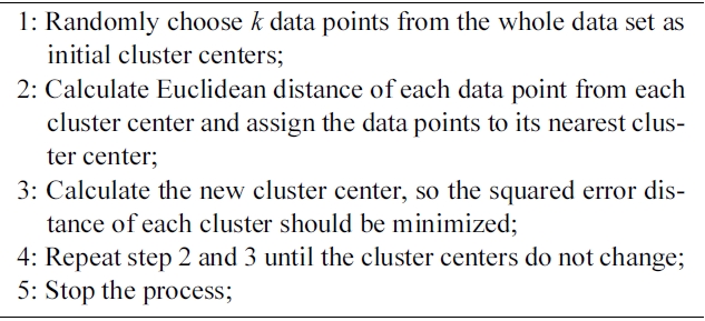
Algorithm 1. K-Means
advance and its computational cost with respect to the number of observations, clusters, and iterations. Although, K-Means is efficient in the sense that only the distance between a point and the k cluster centers ?not all other points? needs to be (re)computed in each iteration. Typically, the number of observations n is much larger than k.
Many approaches have tried to alleviate both these problems.Variations of K-Means clustering that are supposed to cope without prior knowledge of the number of cluster centers have been presented [31, 32]. While the proposed solutions to KMeans clustering certainly improve its practical behavior, they do not overcome the fundamental problems associated with the algorithm.
In [33] density-based algorithms have been proposed as a better alternative to identifying the correct number of clusters in the data. These algorithms make use of Voronoi diagrams (as in[34] and [35]) and are statistically significantly more accurate than K-Means clustering.
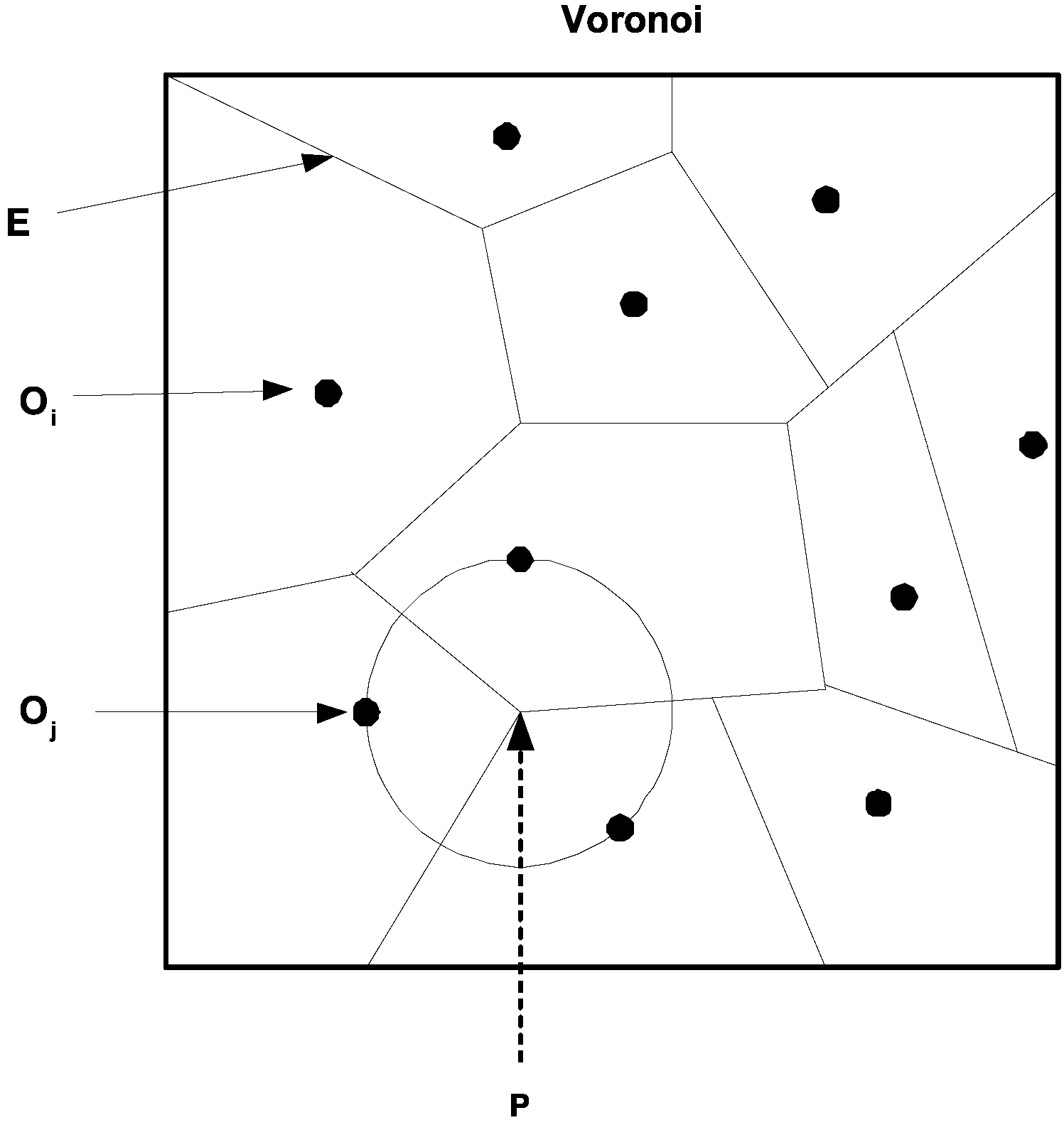
2) Voronoi Diagram:The Voronoi diagram is one of the most important and useful techniques in the field of computational geometry. Given a set D of n data points o1, o2, o3,. . . on in a plane, the Voronoi diagram (V or (D)) is a subdivision of the plane into Voronoi cells (V (oi) for oi) (Fig. 3). The Voronoi cells are the set of points u that are closer to oi than any other point in D. i.e., V(oi) = {u'd(oi, u) ≤ d(oj, u) j ≠ i}, where d is the Euclidian
distance. The Voronoi diagram divides the plane into n convex polygon regions (for each oi), the vertices (P of Fig. 3) of the diagram are the Voronoi vertices, and the borders between two adjacent Voronoi cells are termed Voronoi edges (E of Fig. 3).Note that each Voronoi vertex is the center of a circle touching three or more data points lying in its adjacent Voronoi cells (Fig. 3).
3) Voronoi Clustering:The algorithm presented in [33],begins by constructing the Voronoi diagram for S, where S = s1,. . . , sn ⊆ ?d is a given data set of n points that is going to be clustered. The computational complexity of Voronoi diagram construction in the general case is O(n log n) [36], but requires only linear time in some restricted cases [37]. The algorithm is given as an input parameter a threshold value max indicating the maximum volume allowed to a cell that still can be combined into an evolving cluster.
Each point makes up its own cell in the Voronoi diagram for the data. The volumes (areas in case of the plane) of the cells are computed (or approximated) next. This approximation is not very accurate in small dimensions, but it improves, as the number of dimensions grows. Each cell is associated with a class label. The algorithm assigns increasing integer values as class labels. The point with the smallest Voronoi cell is handled first.
[302] Algorithm 2. Voronoi clustering (set S real max)

Algorithm 2. Voronoi clustering (set S real max)
The cell boundaries in the Voronoi diagram of a point set are by definition equally distant from the relevant points. Thus, the Voronoi diagram naturally gives rise to a kind of maximum margin separation of the data. The algorithm combines existing cells, instead of creating artificial center points as, e.g., KMeans does. Hence, the maximal margins are maintained also in the clustered data. Maximal margin clustering seems a natural choice, since there are no reasons to place the cluster border closer to one or other cluster.
One can view Voronoi clustering as a change of paradigm from the K-Means, whose Euclidean distance minimization can be made autonomous with respect to the number of clusters only by optimizing a parameter that is too hard to learn. Kao et al. [34] proposed a similar pruning technique based on Voronoi diagrams to reduce the number of expected distance calculations in case the mobile objects draw uncertain locations.
IV. TRAJECTORY POLY-LINES AND TWODIMENSIONAL SURFACES
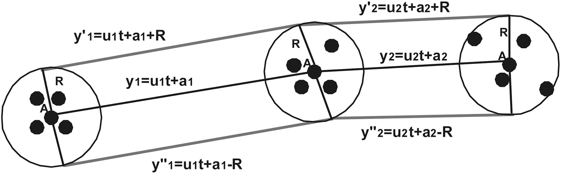
For every mobile user, we calculate a circular range query whose center is its current 2-D location and radius a given value R defined by a minimum circular spatial area
CREATE TABLE Points (
name VARCHAR(20) PRIMARY KEY,
location Point NOT NULL,
description VARCHAR(200),
SPATIAL INDEX(location)
);
To obtain points in a circular area as a counted result ordered by distance from the center of the selection area, we write:
SELECT COUNT(name), AsText(location), SQRT(POW
(ABS(X(location) - X(@center)), 2) + POW(ABS(Y(location)
- Y(@center)), 2)) AS distance
FROM Points
WHERE Intersects(location, GeomFromText(@bbox))
AND SQRT(POW(ABS(X(location) - X(@center)), 2) + POW
(ABS(Y(location) - Y(@center)), 2)) ≤ @R
ORDER BY distance;
If the result returned is less than
Thus, the RQ service depicted in Fig. 2, was transformed to the Privacy-Aware RQ service depicted in Fig. 5:
If the entire buffer lies inside the query area (the buffers of mobile users O3 or O4 in Fig. 5), meaning that both upper and lower boundary poly-lines lie in the query rectangle, then the same holds for the original trajectory. If the entire buffer lies outside the query area (the buffer of mobile user O2 in Fig. 5),meaning that both upper and lower boundary poly-lines lie outside the query rectangle, then the same holds for the original trajectory. In the worst-case, we face the distortion effect, where one of the two boundary poly-lines lies in the query rectangle(the buffer of mobile user O1 in Fig. 5). In the later case, TS(Trusted Server) has to check what happens to the original trajectory.
V. DUALITY TRANSFORMATION OF BOUNDARYTRAJECTORIES AND INFORMATION DISTORTION
The duality transform, in general, maps a hyper-plane
One duality transform for mapping the line with equation
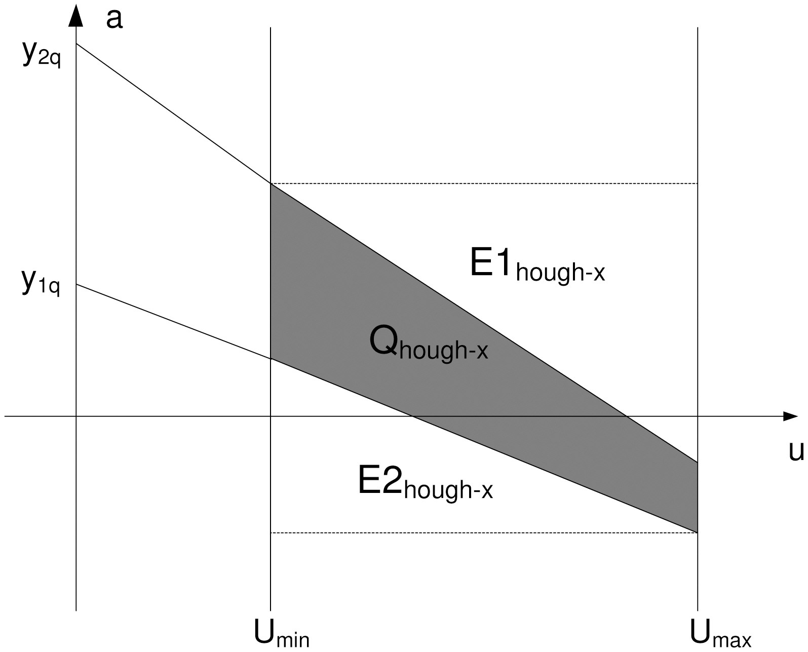
Using a linear constraint query [38], the query in the dual Hough-X plane (Fig. 6) is expressed as:
If u > 0, then QHough-X = A1?A2?A3?A4, where Ai is defined
as follows:
A1 = u ≥ umin,
A2 = u ≤ umax,
A3 = a ≥ y1q ? t2qu,
A4 = a ≤ y2q ? t1qu.
Inequalities of the A1 and A2 areas are obvious. The inequalities for A3 and A4 can be derived as follows: ∀t∈ [t1q, t2q] ⇒ y1q ≤y ≤ y2q ⇒ y1q ? t2qu ≤ y1q ? tu ≤ a ≤ y2q ? tu ≤ y2q ? t1qu, since t1q ≤t ≤ t2q.
If
B1 = u ≤ ? umin,
B2 = u ≥ ? umax,
B3 = a ≥ y1q ? t1qu,
B4 = a ≤ y2q ? t2qu.
Inequalities of the B1 and B2 areas are obvious. For B3 and B4, we are working in the same way as in the case of A3 and A4.
Inequalities of the B1 and B2 areas are obvious. For B3 and B4, we are working in the same way as in the case of A3 and A4.
∀t∈[t1q, t2q] ⇒ y1q ≤ y ≤ y2q ⇒ y1q ? t1qu ≤ y1q ? tu ≤ a ≤ y2q ? tu ≤ y2q ? t2qu, since 0 ≤ t1q ≤ t ≤ t2q and u < 0.
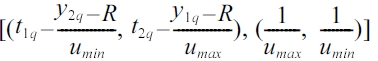
In Fig. 6 the line a = y1q ? t1qu for u = umax becomes a = y1q ? t1qumax and the line a = y2q ? t2qu for u = umin becomes a = y2q ? t2qumin. Thus, for the Service Provider (SP), the initial query [(t1q, t2q), (y1q, y2q)] in the (t, y) plane is transformed to the rectangular query [(umin, umax), (y1q ? t1qumax, y2q ? t2qumin)] in the (u, a) plane.
Similarly, for the upper (y'(t) = ut + a + R) and lower (y''(t) = ut + a ? R) boundary trajectories, SP gets the dual points (u, a + R) and (u, a ? R) as well, as the final (transformed) rectangular queries become [(umin, umax), (y1q ? R ? t1qumax, y2q ? R ? t2qumin)] and [(umin, umax), (y1q + R ? t1qumax, y2q + R ? t2qumin)] respectively in the (u, a) plane.
By rewriting the equation
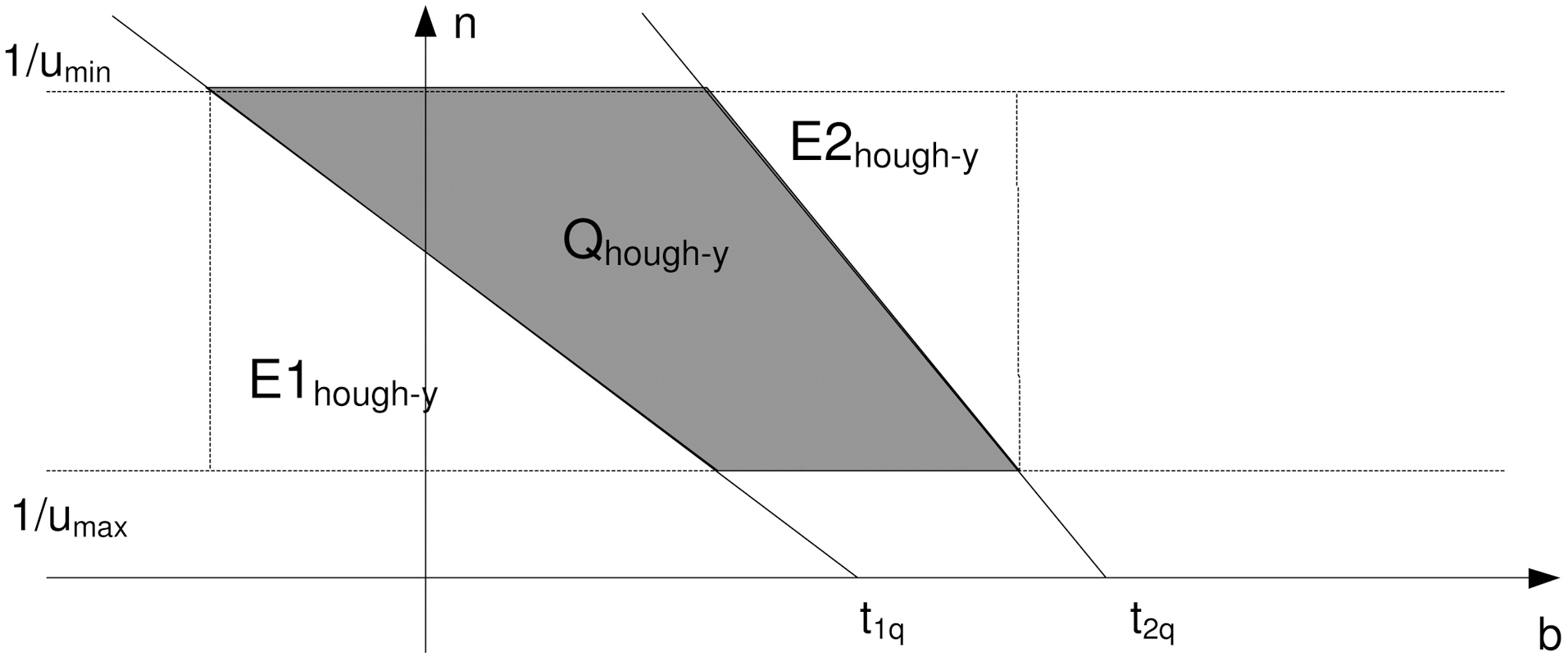
The query in the dual Hough-Y plane (Fig. 7) is expressed as follows. If u > 0, then
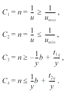
Inequalities of the C1 and C2 areas are obvious. The inequalities for C3 and C4 can be derived as follows: ∀t ∈ [t1q, t2q] ⇒ n =
Hence, the two lines in Fig. 7 have negative slope and for b = 0 intersect the axis b in t1q and t2q, respectively. The intersection of the four regions C1, C2, C3, and C4 form the shaded polygon query of Fig. 7.
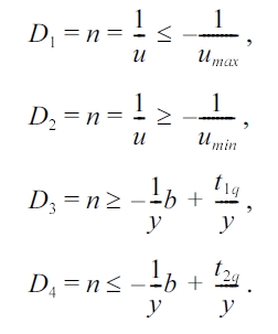
If
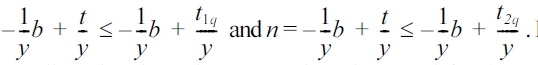
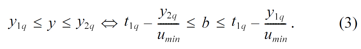
The line n = - 1/y b + t1q/y for = n1/umin iamplies that
In the same way, the line n = - 1/y b + t2q/y for = n1/umin iamplies that
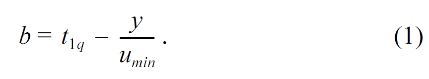
However, according to the initial query and equation (1), we have
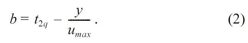
Analogously, according to the initial query and equation (2),we have
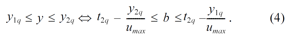
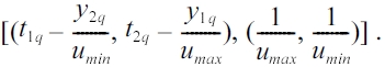
According to (3) and (4) the initial query [(t1q, t2q), (y1q, y2q)] in the (
Similarly,for the upper (
and
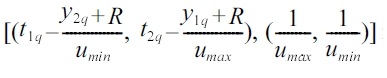
respectively in the (
>
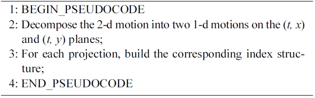
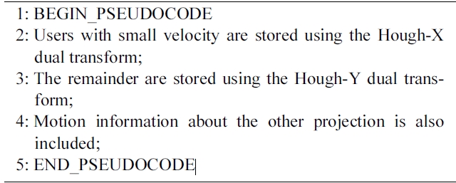
C. The Proposed Algorithm for Privacy-Aware Indexing
Let S = {y1, y2, . . . , yn} be the initial set of original trajectory equations, and S' = { y'1, y''1, y'2, y''2 . . . , y'n, y''n } the set of boundary trajectory equations defined by the buffer.
Then, let HxS = {(u1, a1 + R), (u1, a1 ? R), . . . , (un, ai + R),(un, ai ? R)} and
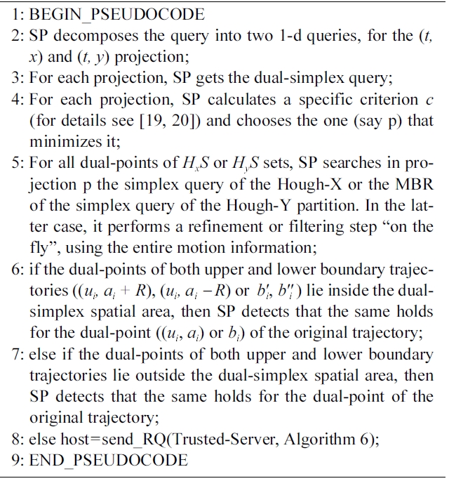
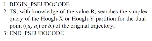
Algorithm 3 runs in SP and depicts the procedure to build the index. Algorithm 4 also runs in SP and presents the procedure to Partition the Mobile Users according to their velocity. Algorithm 5 is running in SP and finally calls Algorithm 6, which is running in Trusted Server (TS) to perform the final filtering step. In particular, Algorithms 5 and 6 outline the privacy-aware algorithm to answer the exact 2-d.
RQ query:
In [19, 20],
In statements 9 and 4 of algorithm 7 and 8 respectively, we call the routine
We define as the motion-pattern of mobile user i at time instant ti the point (
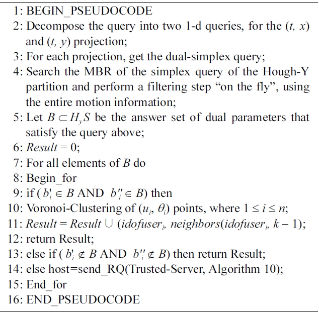
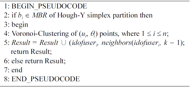
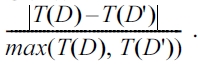
1) Distortion and Competitive Ratio: Let K be the number of bi parameters associated with boundary trajectories of buffers that intersect with the query rectangle. Then, algorithms 9 and 10 require totally T(n) = O(Cost(LazyB_tree) + K) I/Os or block transfers. Moreover, and according to notations presented in[40], let us say that D is the initial Database that stores the N original trajectories and D' the Privacy-Aware Database that stores the 2N boundary-trajectories. Let us also say, Q(D) and Q(D') are the Query Results obtained consuming T(D) and T(D') block-transfers (I/Os) in D and D' database schemes,respectively. We define the Distortion ratio to be the Distortion _Ratio =
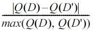
and the
In all cases,
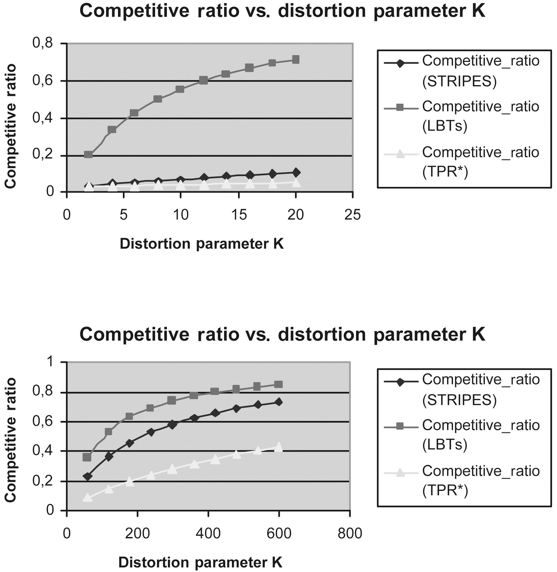
This section compares the query performance of our privacyaware method, when incorporating STRIPES [21] (the best known solution), Lazy B-trees (LBTs) and TPR*-tree, respectively.We deploy spatiotemporal data that contain insertions at a single timestamp 0. In particular, objects’ MBRs are taken from the LA spatial dataset (128971 MBRs) (Downloaded from the Tiger website http://www.census.gov/geo/www/tiger/). We want to simulate a situation in which all objects move in a space with dimensions 100 × 100 km. Thus, each axis of the space is normalized to [0,100000]. For the TPR*-tree, each object is associated with a Velocity Bounded Rectangle (VBR), such that 1) the object does not change spatial extents during its movement,2) the velocity value distribution is skewed (Zipf)towards 30 in range [30,50], and 3) the velocity can be either positive or negative with equal probability. As in [23], we will use a small page size, so the number of index nodes simulates realistic situations.
Thus, for all experiments, the page size is 1 kbyte, the key length is 8 bytes, whereas the pointer length is 4 bytes. Thus,the maximum number of entries (< x > or < y >, respectively) in Lazy B-tree is 1,024 / (8 + 4) = 85. Similarly, the maximum number of entries (2-D rectangles or < x1, y1, x2, y2 > tuples) in TPR*- tree is 1,024 / (4*8 + 4) = 27. Conversely, the STRIPES index maps predicted positions to points in a dual transformed space and indexes this space using a disjoint regular partitioning of space. Each of the two dual planes, are equally partitioned into four quads. This partitioning results in 42 = 16 partitions that we term grids. Thus, the fanout of each non-leaf node is 16. All indexes except STRIPES have similar sizes for each dataset.Specifically, for LA, each tree has 4 levels and around 6700 leaves apart from the STRIPES index that has a maximum height of seven and consumes about 2.4 times larger disk space.Each query
We measured the Competitive Ratio of LBTs method (this method incorporates two Lazy B-trees that index the appropriate
and [22] respectively, using the same query workload, every 10,000 updates.
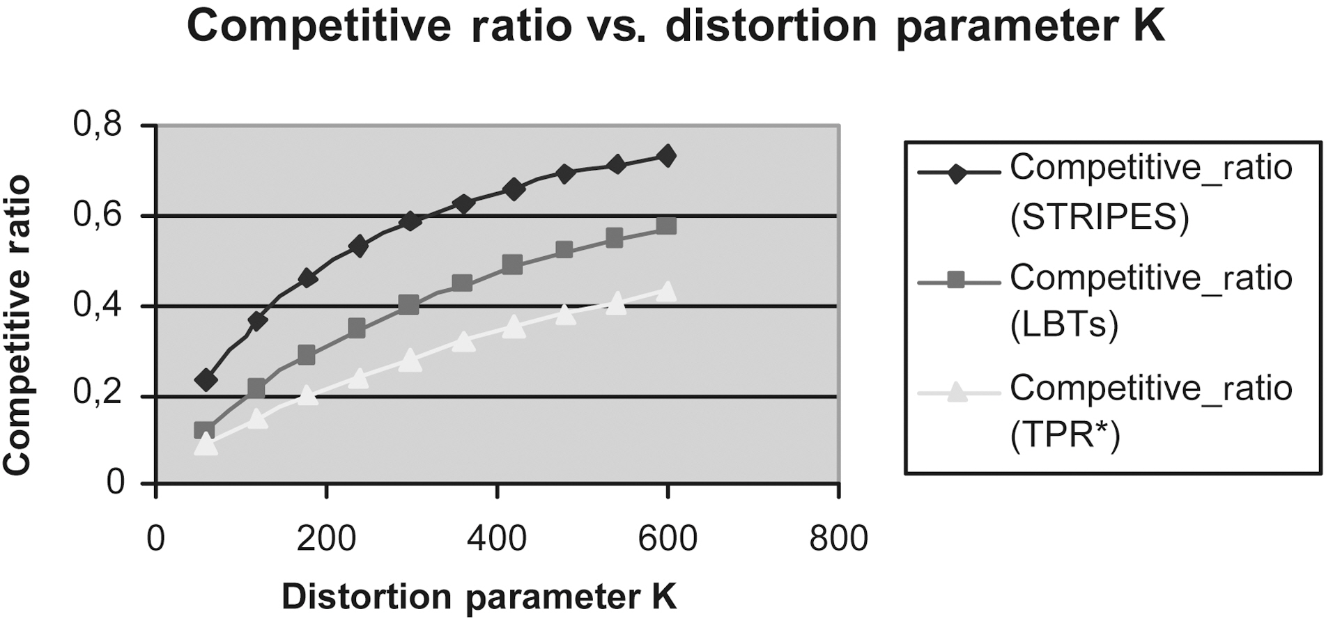
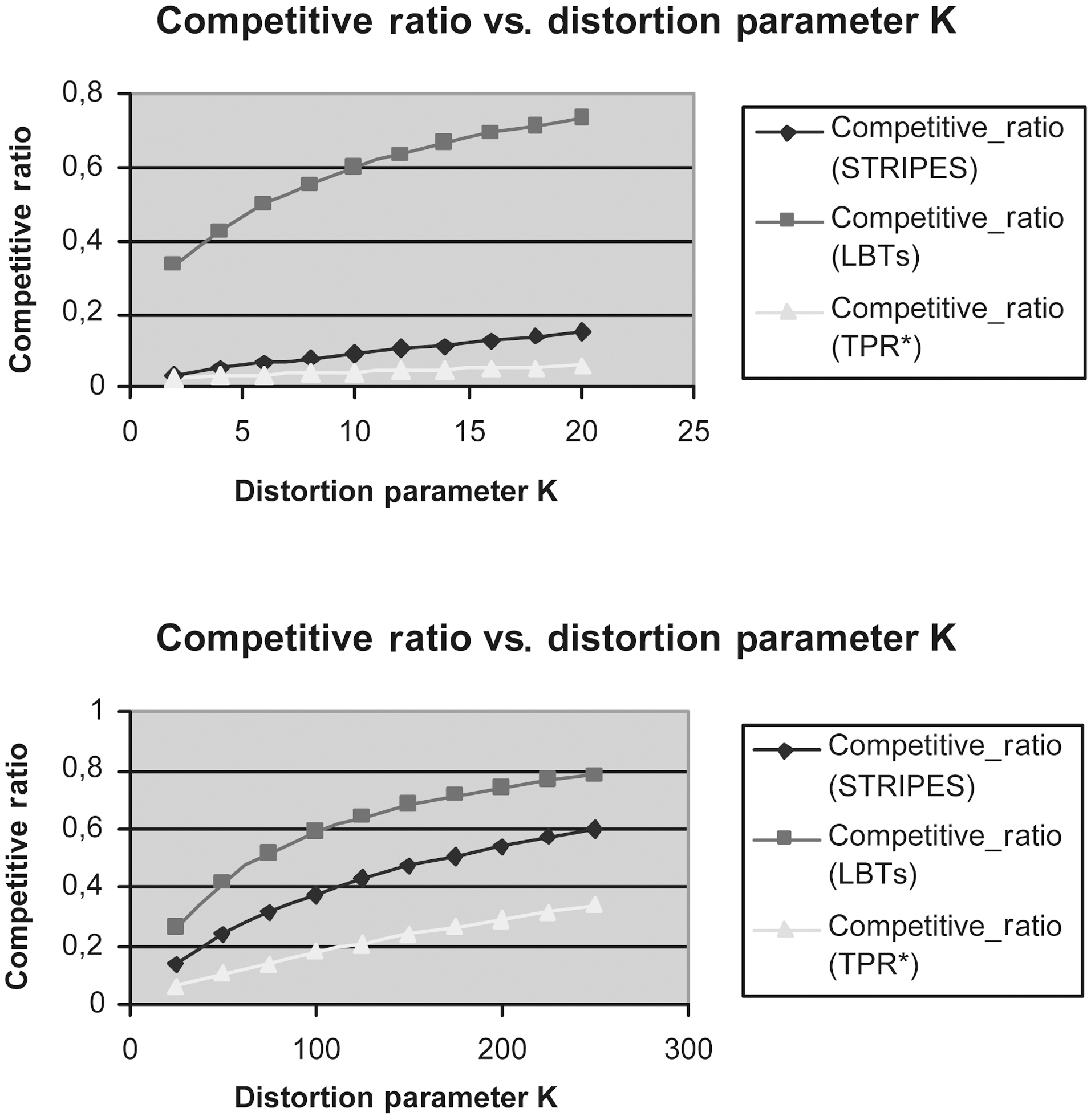
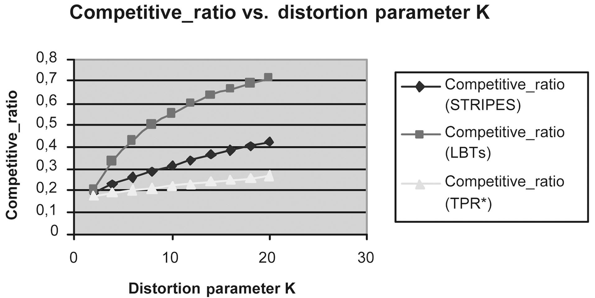
Figs. 9 to 13 show the Competitive Ratio as a function of
depends on the answer’s size, as well as the size of
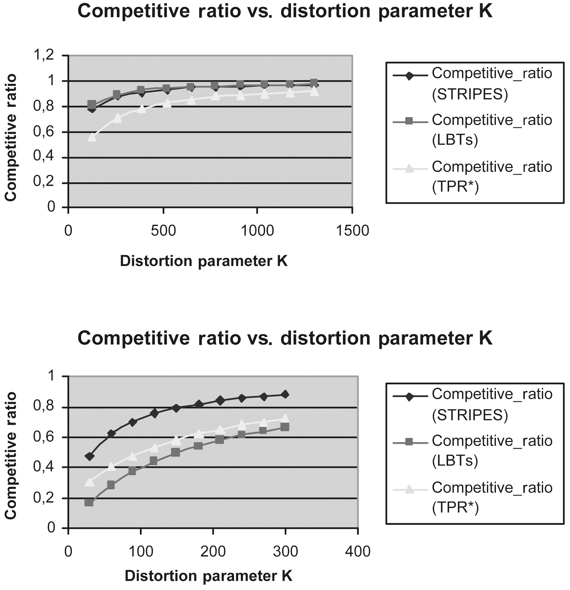
Fig. 12 depicts the performance of all methods where the time interval length degrades to 1. Even in this case, the LBTs method is more competitive than STRIPES and TPR*-tree. As the query rectangle length grows from 400 to 1,000, the LBTs method advantage decreases; we remark that STRIPES becomes faster, whereas LBTs method has exactly the same performance as the TPR*-trees.
Fig. 13 depicts the efficiency of LBTs solution in comparison to that of TPR*-trees and STRIPES, respectively, in the case where the time interval length increases to 100.
We presented the problem of anonymity preservation data publishing in moving objects databases. In particular, we studied the case where the trajectory of a mobile user on the plane is no longer a polyline in a two-dimensional space, instead it is a two-dimensional surface, which covers the real location of the mobile user on the
In this case, the anonymized (kNN) request looks up neighbors,who belong to the same cluster with the mobile requester in (