There has recently been a surge of interest in relational database mining that aims to discover useful patterns across multiple interlinked database relations. It is crucial for a learning algorithm to explore the multiple inter-connected relations so that important attributes are not excluded when mining such relational repositories. However, from a data privacy perspective, it becomes difficult to identify all possible relationships between attributes from the different relations, considering a complex database schema. That is,seemingly harmless attributes may be linked to confidential information, leading to data leaks when building a model. Thus, we are at risk of disclosing unwanted knowledge when publishing the results of a data mining exercise. For instance, consider a financial database classification task to determine whether a loan is considered high risk. Suppose that we are aware that the database contains another confidential attribute, such as income level, that should not be divulged. One may thus choose to eliminate, or distort, the income level from the database to prevent potential privacy leakage. However, even after distortion, a learning model against the modified database may accurately determine the income level values. It follows that the database is still unsafe and may be compromised.This paper demonstrates this potential for privacy leakage in multi-relational classification and illustrates how such potential leaks may be detected. We propose a method to generate a ranked list of subschemas that maintains the predictive performance on the class attribute, while limiting the disclosure risk, and predictive accuracy, of confidential attributes. We illustrate and demonstrate the effectiveness of our method against a financial database and an insurance database.
Commercial relational databases currently store vast amounts of data, including financial transactions, medical records, and health informatics observations. The number of such relational repositories is growing exponentially. Concerns regarding potential data privacy breaches increasingly emerge. One of the main issues organizations face is identifying, avoiding or limiting the inference of attribute values. It is difficult to identify all attribute interrelationships in relational databases due to the size and complexities of database schema that contain multiple relations.
Would it, then, not be enough to eliminate, distort, or limit access to confidential data? Our analysis shows that this is not the case. We show that, when following such an approach, there may still be data disclosure during multi-relational classification.We demonstrate that, through using publicly available information and insider knowledge, one may still be able to inject an attack that accurately predicts the values of confidential,or so-called sensitive, attributes.
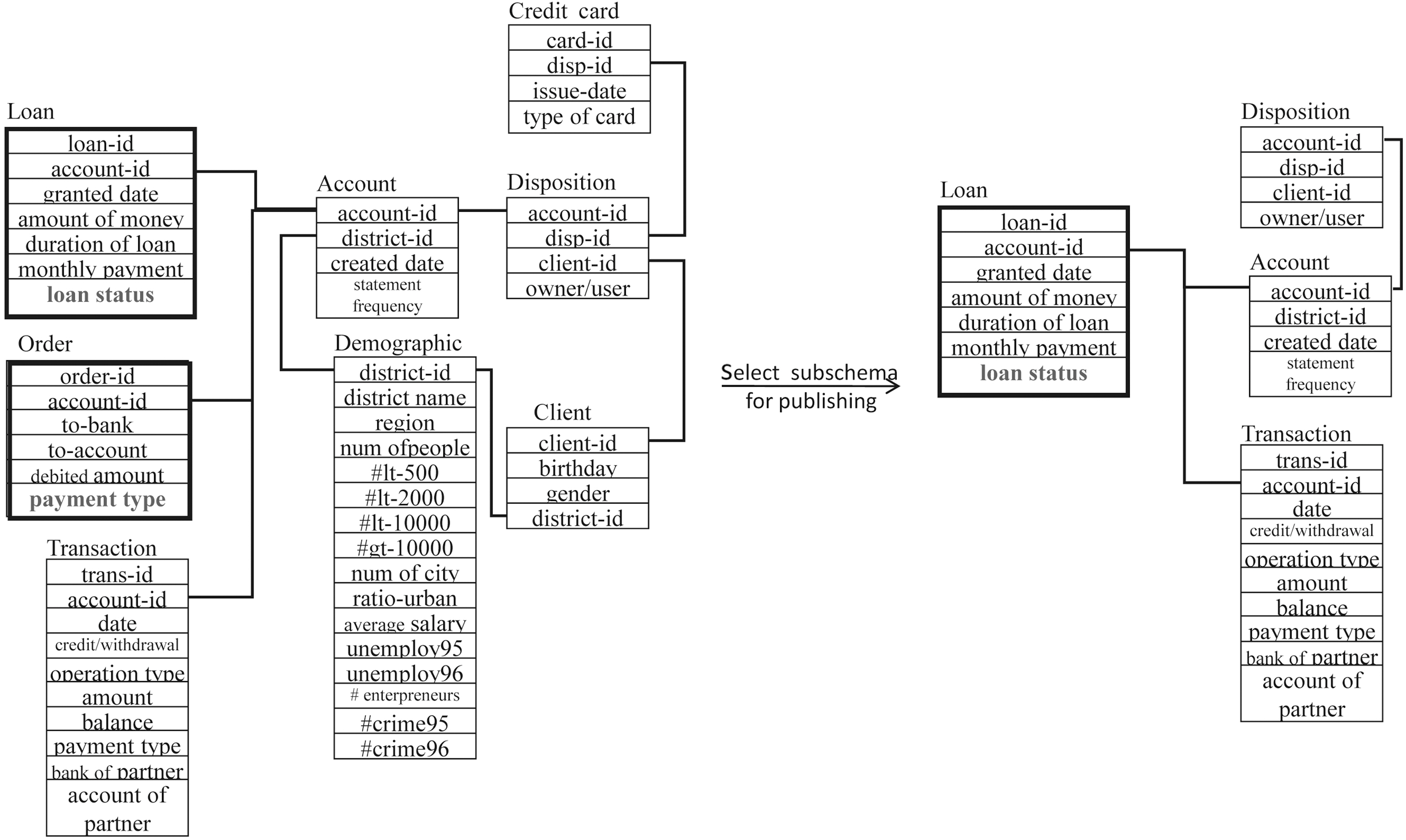
As an example, let us consider the financial database published for the PKDD 1999 discovery challenge [1]. The left subfigure in Fig. 1 shows this database schema. The multirelational classification task here aims to predict a new customer’s risk level, i.e., the loan status attribute (so-called target attribute) in the Loan table, for a personal loan. A loan may be good or bad.The database consists of eight tables. Tables Account, Demographic,Disposition, Credit Card, Transaction, Client, and Order are the so-called background relations and Loan is the target relation. A typical multirelational classification algorithm will identify relevant information (features) across the different relations, i.e., both from the target table and the seven background tables, to separate the good and bad loans in the target relation Loan.
Suppose that we consider the payment type in the Order table as being confidential; it follows that it should be protected. We are interested in protecting the confidential information as to whether a client is paying a home loan. In this example, if the entire database schema is used, one may use a multi-relational classification method, such as the CrossMine approach [2] to predict the loan status in the Loan table with an accuracy of 87.5%. Consider, we shift our target attribute from the loan status in the Loan table to the confidential attribute payment type in the Order table. In this case, we are able to build a CrossMine model to predict if an order is a household payment, with an accuracy of 72.3%. That is, there is a potential for privacy leakage in such a database, if the full database schema is published.
In a worse case scenario, even if we eliminate the payment type from the Order table, an attacker may still be able to partially infer the confidential information based on typical domain knowledge (such as the account holder’s gender) and publicly known statistical data (such as unemployment rates and the number of households in a municipality), or through, for example,assessing the similarity of different objects that tend to have similar class labels [3] or creating tailored accounts in the system[4]. Thus, the attacker can still use the remainder of the database to build a classification model to predict the values of payment type well.
However, suppose we publish a subschema that only consists of tables Loan, Account, Transaction, and Disposition, as shown in the right subfigure in Fig. 1. In this scenario, we are still able to predict a loan’s status with an accuracy of 82.5%. However,here, the predictive accuracy against the sensitive attribute payment type drops from 72.3% to 54.9%, only slightly better than random guessing. The benefit, from a privacy perspective, is high.
Motivated by the above observations, we introduce a method that generates a ranked list of subschemas of a database. Each subschema has a different balance between the two prediction accuracies, namely the target attributes and the confidential attributes. The objective here is to create subschemas that maintain the predictive performance on the target class label, but limit the prediction accuracy on confidential attributes. We show the effectiveness of our strategy against two databases,namely a financial database and an insurance database.
The main contributions of this paper may be summarized as follows.
- We detail a challenge for privacy leakage in multirelational classification. More specifically, we show that by shifting the classification target from the target attributes to confidential attributes, one may be able to predict the values for sensitive attributes accurately.
- We introduce a learning approach, the Target Shifting Multirelational Classification (TSMC) method. The TSMC algorithm generates a ranked list of subschemas from the original database. Each subschema has a different balance between the two prediction accuracies, namely the target attributes and the sensitive attributes.
- We conduct experiments on two databases to show the effectiveness of the TSMC strategy.
This paper is organized as follows. Section II introduces related work. Section III presents the problem formulation. Section IV introduces our method for privacy protection. Section V discusses our experimental studies. Finally, Section VI concludes the paper and outlines our future work.
Privacy leakage protection in data mining strives to prevent revealing sensitive data without invalidating the data mining results [5-8]. Often, data anonymization operations are applied[9].
Current approaches for privacy preservation data mining aim to distort individual data values, while enabling reconstruction of the original distributions of the values of the confidential attributes [5, 10-13]. For example, the k-anonymity model [14]and the perturbation method [15] are two techniques for achieving this goal. In addition, the k-anonymity technique has been extended to deal with multiple relations in a relational database[16].
Recent research deals with correlation and association between attributes to prevent the inference of sensitive data[17-22].For example, Association Rule Hiding (ARH) methods sanitize datasets to prevent disclosure of sensitive association rules from the modified data [17, 19]. Verykios et al. [17] investigate the potential privacy leakage and proposed solutions for sensitive rule disclosure. Zhu and Du [18] incorporate k-anonymity into the association rule hiding process. Tao et al. [20]propose a method to distort data to hide correlations between non-sensitive attributes. Xiong et al. [3] present a semi-supervised learning approach to prevent privacy attacks that make use of the observation that similar data objects tend to have similar class labels.
Data leakage prevention, when releasing multiple views from databases, has also been intensively studied. For example, Yao et al. [23] introduce a method to determine if views from a database violate the k-anonymity principle, thus disclosing sensitive associations that originally exist in the database. In [24], methods for validating the uncertainty and indistinguishability of a set of releasing views over a private table are proposed. In addition,privacy leakage in a multi-party environment has been investigated [25].
This paper details a different direction. Our method does not distort the original data to protect sensitive information. Rather,we select a subset of data from the original database. The selected attributes are able to maintain high accuracies against the target attributes, while lowering the predictive capability against confidential attributes, thus alleviating the risk of probabilistic(belief) attacks of sensitive attributes [9]. This stands in contrast to the above-mentioned anonymization techniques, such as generalization,suppression, anatomization, permutation and perturbation.Furthermore, it follows that our approach is not tied to a specific data mining technique, since there is no need to learn from masked data.
In this paper, a relational database ? is described by a set of tables {R1,· · ·,Rn}. Each table Ri consists of a set of tuples TRi, a primary key, and a set of foreign keys. Foreign key attributes link to primary keys of other tables. This type of linkage defines a join between the two tables involved. A set of joins with m tables R1 ?· · · ?Rm describes a join path, where the length of it is defined as the number of joins it contains.
A multirelational classification task involves a relational database R that consists of a target relation Rt, a set of background relations {Rb}, and a set of joins {J} [26]. Each tuple in this target relation, i.e. x ∈ TRt, is associated with a class label that belongs to Y (target classes). Typically, the task here is to find a function F (x) that maps each tuple x from the target table Rt to the category Y. That is,
Y = F(x, Rt, {Rb}, {J}), x ∈ TRt
Over the past decade, the exponentially growing number of commercial relational databases invoked a surge of interest on multi-relational classification. State-of-the-art multi-relational methods, such as CrossMine [2], TILDE [27], FOIL [28], and MRC [29], have been proposed to effectively and efficiently discover patterns across multiple interlinked tables in a relational database.
We formalize the problem of privacy leakage in multirelational classification, as follows.
A relational database ? = (Rt, {Rb}) with target attribute Y in Rt exists. In addition, we have an attribute C that is to be protected.C ∈ {Rb} (in cases where both Y and C reside in the Rt table, one may create two views from Rt that separate the two attributes into two relations), and C has either to be removed from the database or the values have to be distorted. However,C may potentially be predicted using ? with high accuracy.
Our objective is to find a subschema that accurately predicts the target attribute Y, but yields a poor prediction for the confidential attribute C. To this end, we generate a ranked list of subschemas of ?. Each subschema ?'(?'⊂?') predicts the target attribute Y with high accuracy, but has limited predictive capability against the confidential attribute C. To this end, we construct a number of different subschemas of ?. For each subschema?', we determine how well it predicts the target attribute Y and we calculate its degree of sensitivity in terms of predicting the confidential attribute C. Finally, we rank the subschemas based on this information. In the next sections, we discuss our approach.
IV. TARGET SHIFTING MULTIRELATIONAL CLASSIFICATION
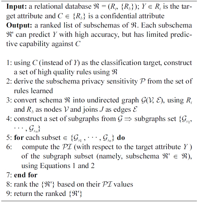
Our Target Shifting Multirelational Classification (TSMC)approach aims to prevent the prediction of confidential attributes,while maintaining the predictive performance of the target attribute. To this end, as described in Algorithm 1, the TSMC method consists of the following four steps.
First, the attributes that are correlated with a confidential attribute are identified. Note that, following Tao et. al, [20] we here use the term correlation to denote the associations, interrelationships or links between attributes in our database. It follows that such correlated attributes may reside in relations other than those containing the confidential attribute. Second, based on the correlation computed from the first step, the degrees of sensitivity for different subschemas of the database are calculated.Next, subschemas consisting of different tables of the database are constructed. Finally, for each subschema, its performance when predicting the target attribute, along with its privacy sensitivity level, is computed. Thus, a ranked list of subschemas is provided. These four steps are discussed next.
>
A. Identify Correlated Attributes Across Interlinked Tables
The aim in the first phase of the TSMC method is to identify the attributes that are correlated with the confidential attribute C. That is, this step finds attributes that may be used to predict C. One needs to compute the correlation between attribute sets across the multiple tables of the database to find correlated attributes. The TSMC method learns a set of high quality rules against the confidential attribute C to address the above issue.That is, it searches attributes (attribute sets) across multiple tables to find a set of rules that predict the values of C. To this end, we employ the CrossMine algorithm that is able to accurately and efficiently construct a set of conjunctive rules using features across multiple relations in a database [2]. The CrossMine method employs a general-to-specific search to build a set of rules to explain many positive examples and cover as few negative ones as possible. This sequential covering algorithm repeatedly finds the best rule to separate positive examples from negative ones. All positive target tuples satisfying that rule are removed after building each rule. The CrossMine strategy evaluates the different combinations of relevant features across relations to build a good rule. The method is able to construct accurate rules that scale by employing a virtual join technique between tables together with a sampling method to balance the number of positive and negative tuples while building each rule. For example, a rule may have the following form:
Loan.status = good ← (Loan.account-id ? Account.account-id) (Account.frequency = monthly) (Account.client-id ? Client.client-id)(Client.birth date < 01/01/1970)
This rule says a monthly loan where the borrower was born before 1970 is classified as being of low risk. In this rule, the attributes frequency in the Account table and birth date from the Client table work together to predict the loan status in the Loan table. That is, such a rule is able to capture the interplay between attributes across multiple tables.
In summary, we use CrossMine to learn which other attributes are correlated, or have a relationship with, the confidential attributes. That is, our approach uses a set of rules as created by this classifier, to identify the most relevant attributes. It follows that an implicit assumption is that an informative classification model is constructed by CrossMine.
The TSMC method ranks the constructed rules based on their tuple coverage and then selects the first n rules that cover more than 50% of the training tuples. That is, the algorithm considers the set of rules that can predict the confidential attributes better than random guessing.
Algorithm 1.TSMC approach
>
B. Assign Privacy Sensitivity to Subschemas
The TSMC method estimates the predictive capability of the subschemas after obtaining a set of rules that finds the other attributes that are relevant when learning the confidential attributes.
Consider the following rule that predicts an order’s payment type in the Order table with 70% accuracy.
Order.payment type = house payment ← (Order.amount ≥1833) (Order.account_id ? Disposition.account_id) (Disposition.client_ id Client.client_id) (Client.birth_date ≤ 31/10/1937)
Thus, if our published subschema includes tables Order, Disposition,and Client, one may use this subschema to build a classification model and then to determine an order’s payment type with an accuracy of 70%.
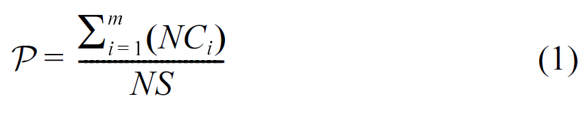
The previous observation suggests that, by using the set of high quality rules learned, we can estimate the degree of sensitivity(denoted as P) of a subschema, in terms of its predictive capability on the confidential attribute. The value of P for a subschema is calculated as follows. First, we identify the set of m ( ) rules whose conjunctive features are covered by some or all of the tables in the subschema. Next, we sum the number of tuples covered by each one of these rules (denoted as NCi). Finally, we divide the sum by the total number of tuples(noted as NS) containing the confidential attributes. Formally,the value P for a subschema is calculated as follows.
For example, as the above-mentioned rule covers 70% of the total number of tuples, we will assign 0.7 as the degree of sensitivity for the subschema {Order, Disposition, Client}. Note that,there may be another rule against this subschema, such as
Order.payment type = house payment ← (Order.amount ≥1833)(Order.account_id ? Disposition.account_id) (Disposition.type= owner)
In this case, the sensitivity of subschema {Loan, Account,and Client} should be calculated using all tuples covered by the two rules. This is due to CrossMine being a sequential covering method, where each of the constructed rules focuses on covering a different portion of all tuples.
The next step of the TSMC method, as described in Algorithm 1, is to construct a set of subschemas and evaluate their contained information, in terms of predicting both the target attribute Y and the confidential attribute C.
The TSMC method adopts the subschema construction approach presented in our earlier work [29]. That is, in the TSMC method, each subschema consists of a set of subgraphs,each corresponds to a unique join path in the relational database.The subgraph construction procedure is discussed next.
1) Subgraph Construction:
The subgraph construction process aims to build a set of subgraphs given a relational database schema, where each subgraph corresponds to a unique join path.The construction process initially converts the relational database schema into an undirected graph, using the relations as the nodes and the joins as edges.
Two heuristic constraints are imposed on each constructed subgraph. The first is that each subgraph must start at the target relation. This constraint ensures that each subgraph contains the target relation and, therefore, is able to construct a classification model. The second constraint is for relations to be unique for each candidate subgraph. Typically, in a relational domain, the number of possible join paths given a large number of relations is very large, making it too costly to exhaustively search all join paths [2]. In addition, join paths with many relations may decrease the number of entities related to the target tuples.Therefore, this restriction was introduced as a trade-off between accuracy and efficiency.
Using these constraints, the subgraph construction process proceeds initially by finding unique join paths with two relations,i.e. join paths with a length of one. These join paths are progressively lengthened, one relation at a time. The length of the join path is introduced as the stopping criterion. The construction process prefers subgraphs with shorter length. The reason for preferring shorter subgraphs is that semantic links with too many joins are usually very weak in a relational database [2,29, 30]. Thus, when considering databases with complex schemas,one can specify a maximum length for the join paths.When this number is reached, the join path extraction process terminates.
After constructing a set of subgraphs, the TSMC algorithm is then able to form different subschemas and evaluate their predictive capabilities on both the target and confidential attributes.
2) SubInfo of Subgraph:
Recall that each subschema consists of a set of subgraphs. We prefer to have a set of subgraphs that are 1) strongly correlated to the target attributes, but 2)uncorrelated with one another, to have better predictive capability for the target attributes. The first condition ensures that the subgraphs can be useful in predicting the target attributes. The second condition guarantees that information in each subgraph does not overlap, when predicting the class. That is, we conduct a form of pruning to identify diverse subgraphs. It follows that all new subschemas that are subsumed by, or highly correlated to, a high risk subschema also poses a risk. Thus, all subschemas should be tested before releasing them to the users to enhance privacy.
We adopted the Subgraph Informative (SubInfo) calculation,as presented in our earlier work [29], to estimate the correlation between subgraphs. In the approach, SubInfo is used to describe the knowledge held by a subgraph with respect to the target classes in the target relation. Following the same line of thought, the class probabilistic predictions generated by a given subgraph classifier is used as its corresponding subgraph’s Sub-Info. Each subgraph may separately be “flattened” into a set of attribute-based training instances by generating relational (aggregated)features. Learning algorithms, such as decision trees [31]or support vector machines [32], may subsequently be applied to learn the relational target concept, forming a number of subgraph classifiers. Accordingly, the subgraph classifiers are able to generate corresponding SubInfo variables.
After generating the SubInfo variable for each subgraph, we are ready to compute the correlation among different subgraph subsets. This is discussed next.
3) Subschema Informativeness:
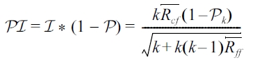
Following the idea presented in our earlier work [29], a heuristic measurement has been used to evaluate the “goodness” of a subschema (i.e., a set of subgraphs), for building an accurate classification model.The “goodness” of a subschema I is calculated as follows.
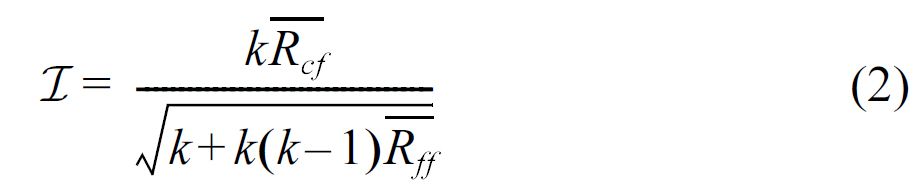
Here, k is the number of SubInfo variables in the subset (i.e.,subschema), Rcf is the average SubInfo variable-to-target variable correlation, and Rff represents the average SubInfo variable-to-SubInfo variable dependence. This formula has previously been applied in test theory to estimate an external variable of interest[33-35]. Hall [36] adapted it to the Correlation-based feature selection (CFS) strategy, where this measurement aims to discover a subset of features that are highly correlated to the class. Also, in our earlier work, as presented in [37], we utilized this formula to select a subset of useful views for multirelational classification.
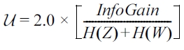
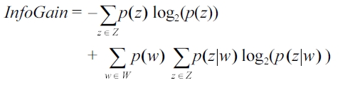
The Symmetrical Uncertainty (U) [38] is used to measure the degree of correlation between SubInfo variables and the target class (Rcf ), as well as the correlations between the SubInfo variables themselves (Rff). This score is a variation of the Information Gain (InfoGain) measure [31]. It compensates for InfoGain’s bias toward attributes with more values, and has been used by Ghiselli [33] and Hall [36]. Symmetrical Uncertainty is defined as follows:
Given variables W and Z,
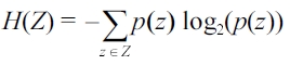
where H(W) and H(Z) are the entropies of the random variables W and Z, respectively. The entropy of a random variable Z is defined as
The InfoGain is given by
4) Subschema Privacy-Informativeness:
We need to consider the predictive capabilities against both the target attribute(represented by I) and the confidential attribute (represented by P) when a database subschema is published to protect privacy leakage. The TSMC method uses a subschema’s PI value to reflect its performance when predicting the target attributes as well as its degree of sensitivity in terms of predicting the sensitive attributes, based on this observation.
The PI value of a subschema is computed using Equations 1 and 2, as follows.
This formulation suggests that a subschema with more information for predicting the target attribute, but with very limited predictive capability on the confidential attribute, is preferred.That is, for privacy protection, a subschema should have a larger I value and a small P value.
5) Subschema Searching and Ranking:
The evaluation procedure searches all of the possible SubInfo variable subsets,computes their PI values, and then constructs a ranking of them to identify a subschema, i.e., a set of uncorrelated subgraphs,which has a large I value but a small P value.
The STMC method uses a best-first search strategy [39] to search the SubInfo variable space. The method starts with an empty set of SubInfo variables, and keeps expanding, one variable at a time. In each round of the expansion, the best variable subset, namely the subset with the highest PI value is chosen.In addition, the algorithm terminates the search if a preset number of consecutive non-improvement expansions occur.
Thus, the method generates a ranked list of subschemas with different PI values. As described in Algorithm 1, the TSMC method calculates such a list. Accordingly, one may select a subschema based on the requirements for the predictive capabilities on both the target attribute and the confidential attributes.
In this section, we demonstrate the information leakage in multirelational classification with experiments against two databases,namely the previously introduced financial database from the PKDD 1999 discovery challenge [1] and the insurance database from ECML 1998 [40]. In addition, we discuss the outputs resulting from the TSMC method to show its effectiveness for privacy leakage prevention in these two multirelational classification tasks. Note that, confidential attributes are removed in these experiments, or distorted, after the application of the TSMC method, since the algorithm first needs to build rules against these attributes. We implemented the PPMC algorithm using Weka version 3.6 [41]. The CrossMine algorithm was obtained from its authors. We ran these experiments on a PC with a 2.66 Ghz Intel Quad CPU and 4 GByte of RAM.
>
A. PKDD’99 Financial Database
In our first experiment, we used the above-mentioned financial database that was offered by a Czech bank and contains typical business data [1]. Fig. 1 shows the database. Recall that,the multirelational classification task aims to predict a new customer’s risk level for a loan. The database consists of eight tables. Tables Account, Demographic, Disposition, Credit Card,Transaction, Client, and Order are the background relations and Loan is the target relation. Our experiment used the data prepared by Yin et al [2].
1) Experimental Setup:
In this experiment, we consider the payment type in the Order table as being confidential and it follows that it should be protected. We assume that the payment type information will either be eliminated from the database, or distorted, prior to being published. The Order table contains the details of an order to pay a loan. It includes the account information,bank of the recipient, account of the recipient, debited amount, and the previously introduced payment type. The payment type attribute indicates one of four types of payments,namely for insurance, home loans, leases or personal loans. In this scenario, more than half of the payments are home loan repayment, i.e. there are 3,502 home loan payment and 2,969 other payment orders. We are interested in protecting the confidential information as to whether a client is paying a home loan.
[Table 1.] Sample rules learned

Sample rules learned
[Table 2.] The number of tuples covered by the set of selected rulesagainst the financial database
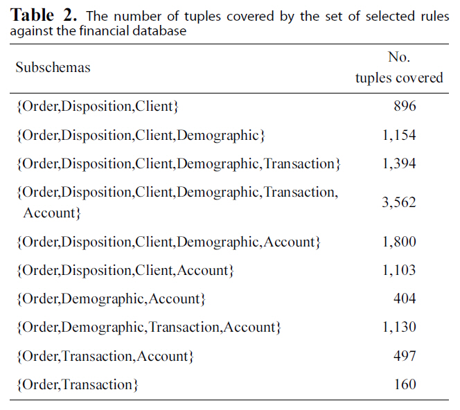
The number of tuples covered by the set of selected rulesagainst the financial database
2) Potential Privacy Leakage:
As a first step, we shifted our target attribute from the loan status in the Loan table to the payment type in the Order table (highlighted in bold in Fig. 1). We used CrossMine to build a classification model [2]. Our experimental results show that we are able to build a set of rules to predict if an order is a household payment with an accuracy of 72.3%. That is, there is a potential for privacy leakage in such a database.
A possible solution here would be to prevent the prediction of the type of payment from the Order table with high confidence,but still maintain the predictive performance against the loan status in the Loan table. The TSMC method is designed to achieve this goal. Next, the execution of the TSMC method against this database is discussed.
[Table 3.] Privacy sensitivity of subschemas against the financial database
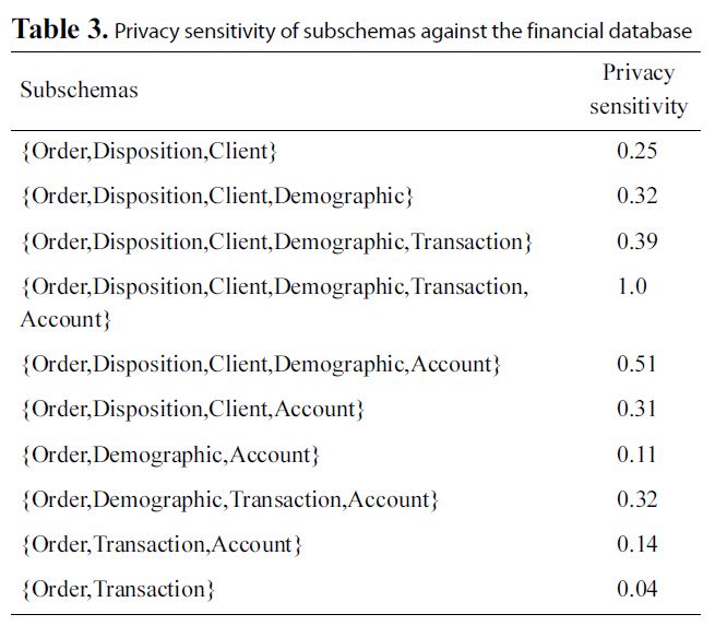
Privacy sensitivity of subschemas against the financial database
[Table 4.] Constructed subgraphs against the financial database

Constructed subgraphs against the financial database
3) Subschema Privacy Sensitivity:
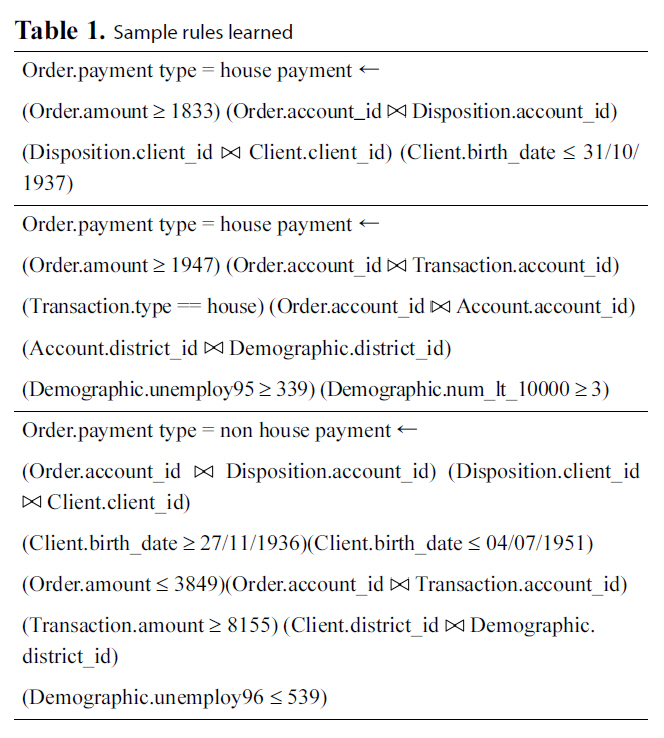
The first step of the TSMC method aims to identify attributes that predict the sensitive attribute, through searching features across multiple tables in the database. 12 high coverage rules were selected from the rules built for predicting the payment type in the Order table.These cover 3,341 instances in the Order table. That is, over 50% of the examples have been covered by the set of rules selected. The aim for the rule selection is to identify attributes(across tables) that are useful to predict the sensitive attribute payment type in the Order table.
For example, Table 1 lists three of the 12 rules learned. The first rule, as described in Table 1, indicates that if a payment with an amount larger than 1,833 in the Order table, and the client,linked through the Disposition table, was born no later than Oct 31, 1937, then it was a home loan payment. This rule involves two attributes that come from different tables. Similarly,the second rule shows that the amount attribute in the Order table works together with the type attribute in the Transaction table. The rule also indicates that the level of unemployment in 1995 and the number of municipalities with between 2,000 and 9,999 inhabitants in the Demographic table are of importance to categorize the values for the payment type in the Order table. The same idea was demonstrated by the third rule that includes attributes birth date in the Client table, amount in the Order table, amount in the Transaction table, and the level of unemployment in 1996 from the Demographic table. Importantly,these rules indicate that publicly known statistical data,such as unemployment rates and the number of households in a municipality, may be used to inject attacks when aiming to target individuals. That is, an attacker may be able to infer confidential information from the data mining results through the combination of public and insider knowledge.
These rules show how attributes across tables work together to predict the confidential attributes. That is, these rules were able to capture the correlation and their predictive capability among multiple attributes across multiple tables, regardless of the attribute types.
As described in Algorithm 1, the second step of the TSMC method is to identify the privacy sensitivity of different subschemas.Let us reconsider the first conjunction rule, as shown in Table 1. If we evaluate this rule at the table level, we may conclude that the subschema which consists of the tables{Order, Disposition, Client} has attributes to construct this rule.Thus, we may want to avoid using this subschema or, at least,restrict access to it.
The privacy sensitivity of a subschema is computed using Equation 1, as described in Section IV-B. Accordingly, from the tuple coverage of Table 2, we calculate the degree of sensitivity for each subschema using Equation 1, and present the results in Table 3. As shown in Table 3, different subschemas have various privacy sensitivities, in terms of predicting the confidential attribute payment type in the Order table. For example, the subschema that consists of tables {Order, Disposition, Client,Demographic, Transaction, and Account} has the highest privacy sensitivity. That is, this subschema may be used to build an accurate classification model to determine the value of an order’s payment type.
We are able to construct and select different subschemas with various privacy sensitivities against the confidential attributes
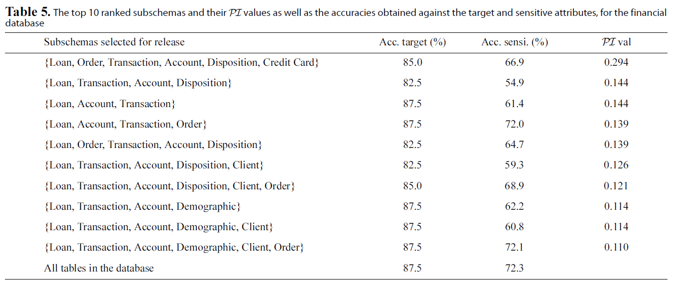
The top 10 ranked subschemas and their PI values as well as the accuracies obtained against the target and sensitive attributes for the financialdatabase
and predictive capability for the target attributes, with the degrees of privacy sensitivity of different subschemas of the provided database. We will discuss these two elements in detail next.
4) Subschema Evaluation:
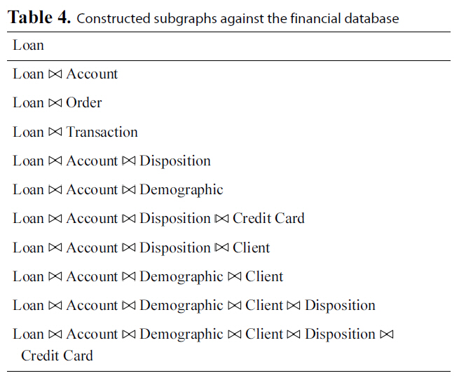
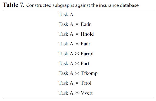
Following the strategy as described in Section IV-C, we construct the set of subgraphs from the provided database. Each subgraph corresponds to a join path starting with the target table. Eleven subgraphs were constructed by the TSMC method. The subgraphs are presented in Table 4.
After constructing the subgraphs, the search algorithm computes different combinations of subgraphs, resulting in different subschemas. Consequently, each subschema has a PI value that reflects information about the target attribute classification, as well as the predictive capability against the confidential attributes.That is, a ranked list of subschemas, each with a measurement describing the trade-off between the predictive capability against the target attribute and confidential attribute, is created.Table 5 presents the top ten subschemas generated from the financial database. In this table, we show the tested results against the target label (i.e., the loan status), as well as the confidential attribute (namely, the payment type). We provide the accuracy obtained against the full database schema at the bottom of the table for comparison.
One can see from Table 5 that the TSMC method has created a list of subschemas with different predictive capability against the target attribute and the confidential attribute. The experimental results, as shown in Table 5, suggest that one may select a subschema with a good trade-off between the two predictive capabilities.
Specifically, one is able to identify the dangerous subschemas that pose a high data leakage risk. For example, in Table 5,consider the subschema containing tables {Loan, Transaction,Account, Demographic, and Client}. In this case, the accuracy against the target attribute remains the same as against the full database schema. However, the accuracy drops from 72.3% to 60.8% for the confidential attribute. It follows that it is up to the owner of the database to decide if this potentially high level of leakage is acceptable. Conversely, one may prefer to publish the
subschema with tables {Loan, Transaction, Account, and Disposition}to have more confidence in protecting the sensitive attribute. One is able to predict the confidential payment type in the Order table with an accuracy of 54.9 % using this subschema.It follows that this value is only slightly better than random guessing. However, this subschema still predicts the target attribute, namely the loan status from the Loan table with an accuracy of 82.5%, slightly lower than the 87.5% against the original, full database.
In summary, the experimental results show that the TSMC method generates a ranked list of subschemas with different trade-offs between multirelational classification accuracy and predictive capability against confidential attributes.
>
B. ECML’98 Insurance Database
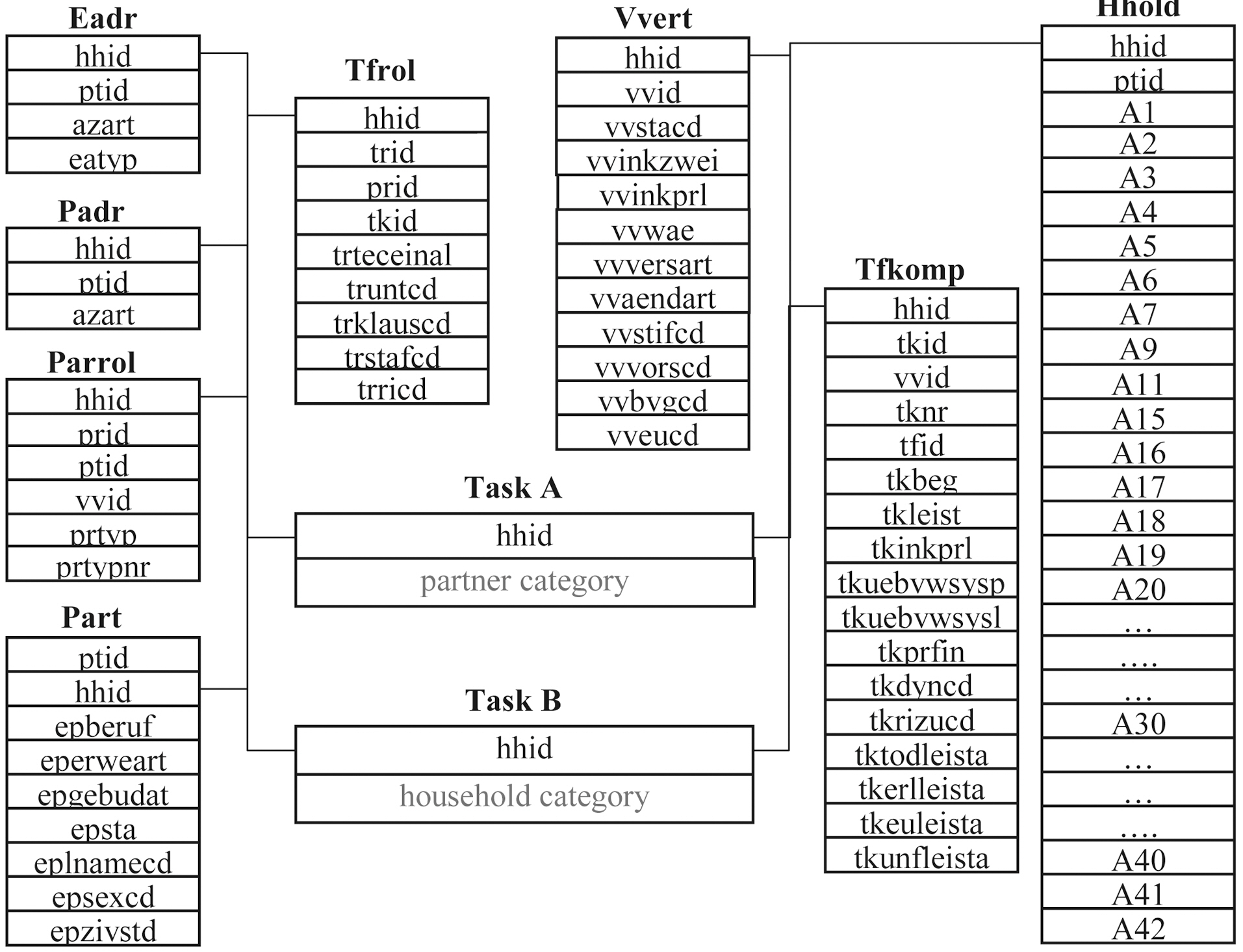
Our second experiment used the database provided for the ECML 1998 challenge [40]. This database was extracted from a data warehouse of a Swiss insurance company. Originally, two learning tasks, namely tasks A and B were presented from this database. Task A is to classify the partner category into 1 or 2.Task B categorizes the household category of class positive or negative. These two tasks are included in tables Task A and Task B, respectively. Eight background relations are provided for the two learning tasks. They are stored in tables Part, Hhold,Eadr, Padr, Parrol, Tfkomp, Tfrol, and Vvert, respectively. The Part table contains the partners of the insurance company. Most of these partners are customers. Partners’ household information is collected into the Hhold table and their addresses are described in the Eadr and Padr tables. In addition, tables Parrol,Tfkomp, Tfrol, and Vvert contain partners’ insurance information.
1) Experimental Setup:
In this experiment, we used the new star schema of the ECML 1998 database, as prepared in [40]. In addition, we removed attributes that contain missing values from the original database, to avoid finding appropriate methods to fill these missing categorical or numerical values. Fig. 2 depicts the resulting database schema. In addition, we suppose that the multirelational classification task here aims to classify partner category in the Task A. We consider the household category in Task B as being confidential and it follows that it should be protected. That is, we are interested in protecting the confidential information as to whether a household category is positive. This database includes 3,705 positive households and 3,624 negative ones.
2) Experimental Results:
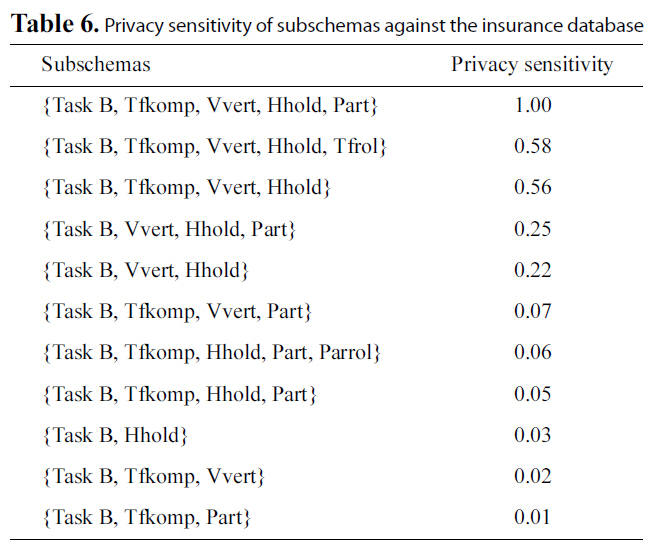
The collected subgraphs and the privacy sensitivities of different subschemas constructed by the TSMC method for the ECML database are presented in Table. 6 and 7, respectively. In addition, we provided the top ten subschemas generated from this insurance database in Table 8. In this table, we show the tested results against the target label(i.e., the partner category), as well as the confidential attribute(namely, the household category). We provide the accuracy obtained against the full database schema at the bottom of the table for comparison.
Results from the last row of Table 8 indicate that there is a potential for privacy leakage in such a database, given that the
130
[Table 6.] Privacy sensitivity of subschemas against the insurance database

Privacy sensitivity of subschemas against the insurance database
[Table 7.] Constructed subgraphs against the insurance database

Constructed subgraphs against the insurance database
full database schema is published for multirelational classification tasks. In this case, we are able to build a CrossMine model to predict if a household is positive with an accuracy of 69.5%.That is, we can use the published database to predict the values
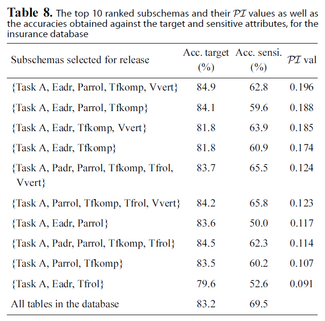
The top 10 ranked subschemas and their PI values as well asthe accuracies obtained against the target and sensitive attributes for theinsurance database
of the household category attribute.
The TSMC method has created a list of subschemas with different predictive capability against the target attribute and the confidential attribute to cope with such potential data leakage.The experimental results, as shown in Table 6, suggest that one can select a subschema with a good trade-off between the two predictive capabilities. For example, in Table 8, consider the subschema containing tables {Task A, Eadr, Parrol, and Tfkomp}.In this case, the accuracy against the target attribute is slightly higher than that against the full database schema, and accuracy against the confidential attribute drops about 10% (from 69.5%to 59.6%). Alternatively, one may prefer to publish the subschema with tables {Task A, Eadr, Parrol} to have more confidence in protecting the sensitive attribute. One is able to predict the confidential household category in the Task B table with an accuracy of only 50.0% using this subschema. It follows that this value is not better than random guessing. Nevertheless, this subschema still predicts the target attribute, namely the partner category from the Task A table with an accuracy of 83.6%,which is slightly higher than the 83.2% against the original, full database. These experimental results show that the TSMC method is able to generate a ranked list of subschemas with different trade-offs between the multirelational classification accuracy and the predictive capability against the confidential attributes.
Importantly, the experimental results, as shown in Table 8,indicate that one is able to identify the dangerous subschemas that pose a high data leakage risk. For instance, the subschema containing tables {Task A, Padr, Parrol, Tfkomp, Tfrol, and Vvert} and the subschema containing {Task A, Parrol, Tfkomp,Tfrol, and Vvert} can be used by the CrossMine method to predict the sensitive attribute household category with an accuracy of over 65%. That is, these subschemas can be used to attack the confidential attribute with accuracy only slightly lower than that against the original, full database. Conversely, the subschema containing tables {Task A, Eadr, and Parrol} and the subschema
[Table 9.] Parameters for the data generator

Parameters for the data generator
containing tables {Task A, Eadr, and Tfrol} can predict the value of a household’s category with an accuracy of only about 50%. It follows that it is up to the owner of the database to decide if a certain level of potential leakage is acceptable.
In summary, our experimental results against the PKDD financial and ECML insurance databases show that the TSMC method generates a ranked list of subschemas with different trade-offs between the multirelational classification accuracy and the predictive capability against the confidential attributes.In particular, the TSMC method is able to identify the dangerous subschemas that pose a high data leakage risk.
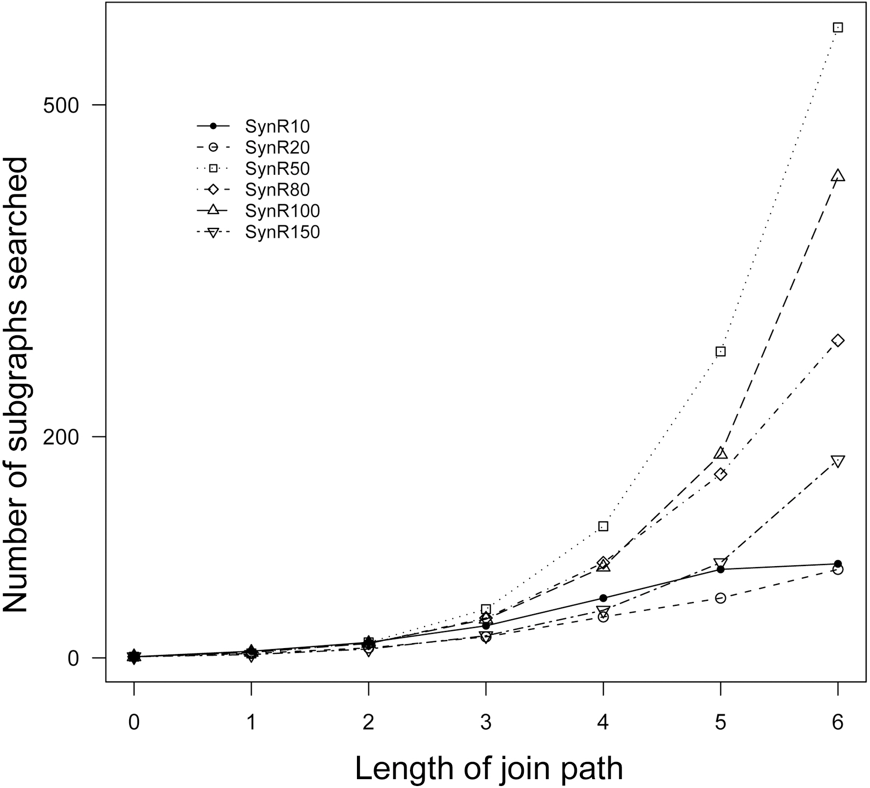
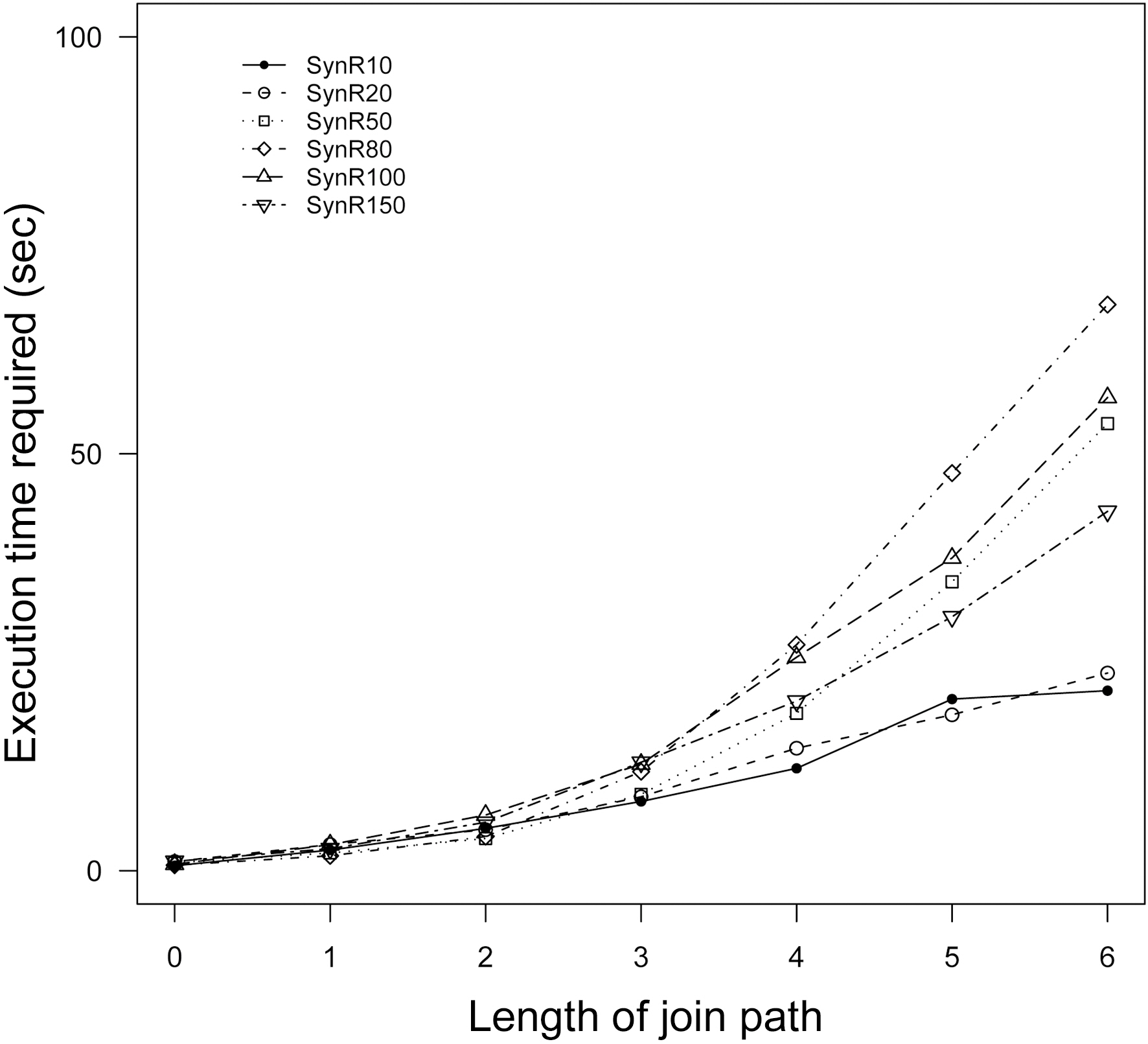
The computational cost of the TSMC algorithm heavily depends on the subschema evaluation procedure, as depicted in Section IV-C. We generated six synthetic databases with different characteristics to evaluate the scalability of the TSMC method against complex databases. The aim of these experiments was to further explore the applicability of the TSMC algorithm when considering relational repositories with a varying number of relations and tuples.
1) Synthetic Databases:
The database generator was obtained from Yin et al. [2]. In their paper, Yin et al. used this database generator to create synthetic databases to mimic real-world databases to evaluate the scalability of the multirelational classification algorithm CrossMine. The generator first generates a relational schema with a specified number of relations to create a database. The first randomly generated table was chosen from these as the target relation and the others were used as background relations. In this step, a number of foreign keys is also generated following an exponential distribution. These joins connect the created relations and form different join paths for the databases. Finally, synthetic tuples with categorical attributes(integer values) are created and added to the database schema.Users can specify the expected number of tuples, attributes,relations, and joins, etc., in a database to obtain various kinds of databases using this generator. Interested readers are referred to the paper presented by Yin et al. [2] for a detailed discussion of the database generator.
The expected number of tuples and attributes were set to 1,000 and 15, respectively, for each of the generated databases. Default values, as found in Yin et al. [2], were used for the other parameters of the data generator. Table 9 lists the most important parameters. The six databases were generated with 10, 20,50, 80, 100, and 150 relations (denoted as SynR10, SynR20,SynR50, SynR80, SynR100, and SynR150), respectively. We ran these experiments on a PC with a 2.66 Ghz Intel Quad CPU and 4 GByte of RAM.
2) Experimental Results:
Recall from Sections V-A and V-B that, for the financial and insurance databases, each subschema in the TSMC method consists of up to 11 subgraphs. In our experiment here, we varied the join path length, as defined in Section III, from zero to six, against each of the six synthetic databases. That is, we allowed a subgraph, i.e., a join path, to contain up to seven tables. Thus, the number of subgraphs to be evaluated by the TSMC algorithm for each database increases substantially. For example, the number of subgraphs for the
SynR50, SynR80, and SynR100 databases are 570, 287, and 435, respectively, when the join path length is six. More details can be found in Fig. 3. The run time required to complete the calculation (in seconds) for each of the databases and the number of subgraphs collected by the TSMC approach are shown in Figs. 3and 4, respectively.
The experimental results, as presented in Figs. 3 and 4, indicate that, even though the number of subgraphs that has to be explored by the TSMC approach increases quasi exponentially,with respect to the join path length in databases with a large number of relations and tuples, the execution time required for the TSMC algorithm increases much less rapidly. For example,as shown in Fig. 3, for the SynR50 database, the number of subgraphs explored by the TSMC strategy jumped from 44 to 119,and then to 570 when the length of join paths allowed were set to 3, 4, and 6, respectively. However, the run time associated with these processes was 10, 19, and 50 seconds, respectively.Similar results are observed with the remaining five databases.Importantly, for all six databases, although the number of subgraphs explored by the TSMC method is very large, the execution time required by the TSMC approach is relatively small. In conclusion, these experimental results suggest that the TSMC strategy scale relatively well in term of run time when applied to complex databases.
VI. CONCLUSIONS AND DISCUSSIONS
Relational databases have been routinely used to collect and organize much real-world data, including financial transactions,medical records, and health informatics observations, since their first release in 1970s. Mining such repositories offers a unique opportunity for the data mining community. However, it is difficult to detect, avoid and limit the inference capabilities between attributes for complex databases, especially during data mining. This is due to the complexity of the database schema,the involvement of multiple interconnected tables and various foreign key joins, thus resulting in potential privacy leakage.
This paper proposed a method to generate a ranked list of subschemas for publishing to address the above-mentioned challenge. These subschemas aim to maintain the predictive performance on the target attribute, but limit the prediction accuracy against confidential attributes. Thus, the owner of the database may instead decide to publish one of the generated subschemas that have an acceptable trade-off between sensitive attribute protection and target attribute prediction, instead of the entire database. We conducted experiments on a financial database and an insurance database to show the effectiveness of the strategy. Our experimental results show that our approach generates subschemas that maintain high accuracies against the target attributes, while lowering the predictive capability against confidential attributes.
Several future directions would be worth investigating. First,as stated earlier, our approach uses a set of rules built by a classifier to detect those attributes that are correlated with a sensitive attribute. We aim to investigate other ways to detect such correlations. For example, it would be interesting to study methods that are able to directly compute the attribute correlations across multiple tables effectively, instead of relying on specific classification or association analysis algorithms. Second, research suggests that relations that are closer to the target relation play a more important role while building an accurate multi-relational classification model [30]. We intend to integrate these findings in our further studies.
Finally, many real world databases contain many confidential attributes, instead of only one. Further studies on extending the proposed approach in this paper to deal with multiple attributes would be very useful. For instance, when multiple sensitive attributes are independent of one another, we may be able to repeat the TSMC approach and incorporate a subschema’s different sensitivities (against different confidential attributes) in Equation 1, through, for example, using the maximum value. A potential problem here is that if the number of confidential attributes is large, we may have difficulty to find a subschema that satisfies the protection for all confidential attributes. However,we may be in a better position to find a good subschema when considering multiple correlated confidential attributes. In such a scenario, one of the challenges would be to make use of the correlations between the multiple confidential attributes. For instance, one may be able to re-use the results computed for the previous attribute (attributes), thus speeding up the search process.
Our algorithm generalizes to multiple sensitive attributes with, at most, linear complexity in terms of computational cost.Let us suppose, for illustration, that we want to add one more sensitive attribute; the generalization to multiple attributes is immediate. Two cases need to be considered. That is, the two attributes are either highly correlated or they are weakly or uncorrelated. In the first case, one may simply re-use the results obtained from the calculation associated with the first attribute,since both attributes are highly correlated. In the second scenario,the calculations are simply repeated for the second attribute. It follows that the outcomes of both calculations are independent, since both attributes are statistically independent.The complexity of such an operation is linear due to the independence of the two attributes.