Magnetic field dipolarization is a sudden change of the magnetic field structure from a stretched configuration(tail-like) to a dipolar configuration in the magnetotail, and is usually observed associated with substorm occurrence in the Earth’s magnetosphere-ionosphere system(Park et al. 2010). Often, the dipolarization process is characterized by complex fluctuations, the turbulent nature of which has only been studied to a limited extent.Magnetic turbulence is important because it could possibly influence the transport and acceleration of plasma particles in association with substorms, and could shed some light on related plasma instabilities, the details of which, however, are largely unknown. The origin of such turbulence is also a fundamental question, as it can be due either to internal instabilities in the near-Earth tail, or to flow activities associated with mid-tail magnetic reconnection.

There are several papers on turbulence in the Earth’s plasma sheet. A preliminary assessment on turbulence in the Earth’s plasma sheet was made by Borovsky et al.(1997). The study included an overall description on a variety of aspects of turbulence in the plasma sheet, but detailed explanations on many issues were left unanswered.Borovsky & Funsten (2003) later extended the work to achieve an improved understanding of turbulence in the plasma sheet. Both papers include discussions on turbulence of both plasma flows and the magnetic field. Angelopoulos et al. (1999) found that the plasma flows in the plasma sheet are intermittent in nature. The magnetic field turbulence has been also studied. Using multi-spacecraft observations from Cluster, Weygand et al. (2005) were able to estimate turbulent eddy scale sizes in association with magnetic field fluctuations in the plasma sheet. Voros et al. (2004) introduced a wavelet technique to study magnetic turbulence, as obtained from the same Cluster satellite observations. In the work by Shiokawa et al. (2005), the power spectral indices were determined for magnetic fluctuations during near-Earth tail dipolarizations. The determination was done for the magnetic field magnitude fluctuations in the frequency range from 0.01 Hz to ~10 Hz, and the results show a steeper slope at a higher frequency regime.

Our goal in this study is to determine the degree of the anisotropic nature of the magnetic turbulence associated with magnetic dipolarizations in the plasma sheet. This has not been reported in any of the previous works on the Earth’s magnetospheric physics. For this study, we identified a total of 47 dipolarization events in a one month period, February 2008, using the magnetic field observations by the three near-tail satellites, THEMIS A, D and E, when they were situated close to the neutral sheet. For the 47 events, we performed fast Fourier transform (FFT) power spectral analysis to estimate the spectral indices in the frequency regime from 1.3 mHz to 42 mHz, and compared them to determine the extent to which they can be anisotropic in a statistical sense.

First, we identified magnetic dipolarization events by using the magnetic field data provided at spin time resolution of 3 seconds, from the three THEMIS spacecraft,A, D and E, when they were at near-tail, X ~ -7 to -12 R_E. To ensure close proximity of the satellites to the neutral sheet, we required that the average Bx to Bz ratio be less than 1 around the dipolarization onset time. For this study, a well-defined dipolarization was based on the requirement that Bz increase by 3 nT or more, or that the magnetic elevation angle increase by 10 deg or larger within 10 minutes after onset. However, since these simple criteria could lead to a false dipolarization, we checked all of the identified dipolarizations visually to determine whether they actually looked like a typical substorm-associated dipolarization. Based on this set of criteria, we identified a total of 47 events in February 2008.

In this paper, we define a local coordinate system in which the three components of the magnetic field are decomposed into the parallel component, δB_II, and the two perpendicular components, δB_φ and δB_ψ, with respect to the background magnetic field. Here, the φ component refers to the azimuthal direction in the usual spherical coordinate system, and the ψ component completes the right-handed orthogonal coordinate system. The ψ coordinate refers to the poloidal flux coordinate. The use of the two perpendicular components, δB_φ and δB_ψ, can be useful in terms of understanding the polarization on the perpendicular plane, which can give a hint to the mode structure of instability during the fluctuations. Also, “δ” refers to the detrended values, which were obtained by applying a 5^th order polynomial fitting to the original data to obtain a trend (which is taken as a background field). We have calculated the spectral power densities based on the typical FFT method for the three components, δB_II, δB_φ and δB_ψ, for the 47 events. From this, we have determined the power spectral indices, α, for the three components, by applying least-square fits to the power spectral densities in log-log space, which are assumed to be of a form f^-α, in which f refers to frequency.

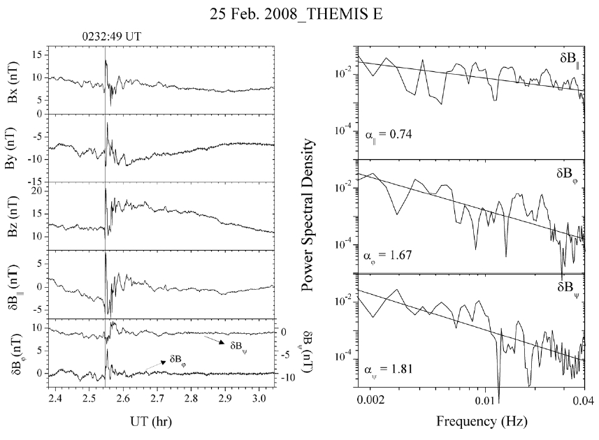
Fig. 1 shows the magnetic field data (left) and the corresponding power spectral density (right) for an example event obtained from the THEMIS E observations on February 25, 2008. The original x, y, and z components, as well as the detrended components, δB_II, δB_φ and δB_ψ, of the magnetic field, are shown in the left panels. The power spectra were obtained by applying FFT to the 40 min time interval shown in the left panels (10 minutes before and 30 minutes after the dipolarization onset, as marked by the vertical line). From the power spectral curves, the spectral indices α for each magnetic component were estimated. In doing this, we have limited the fitting to the frequency range, 1.3 mHz up to 42 mHz (More discussion on this point is given in the last section). The values of α_II, α_φ and α_ψ for δB_II, δB_φ and δB_ψ are 0.74, 1.67, and 1.81, respectively, as indicated in the right panels, and thus, α_ψ > α_φ > α_II. This is an indication of the anisotropic spectral behavior of the magnetic turbulence.

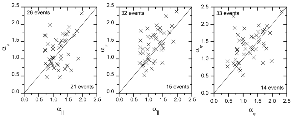
We performed a similar analysis for all of the 47 dipolarization events in the same manner as described above, and obtained the spectral power profiles and the associated spectral indices. The statistical results are analyzed in two different ways, as presented in Figs. 2-4. First, Fig. 2 shows the scatter plots of the spectral indices α for all of the 47 events. The indices are presented for three pairs of two different components, so that a degree of anisotmulti

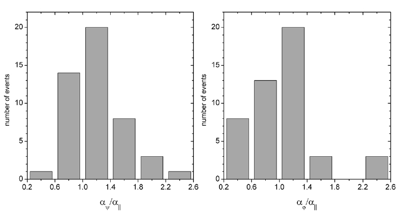
ropy can be judged by visual observation. Note that a diagonal line is drawn in each panel to refer to the line of the isotropic values for a given pair of the indices; if the indices for the pair are the same for all of the 47 events, they should all lie on the diagonal line. For all of the three pairs, however, there are events off this line, implying some degree of anisotropy. For the pair α_φ and α_II, which is shown in the left panel, there is a slightly higher number of events (26 events) showing α_φ > α_II, than the opposite case (21 events). The middle panel shows that ~68% (32 events) of the 47 events are associated with a larger α_ψ than α_II. For the pair between α_ψ and α_φ (right panel), ~70% (33 events) of the 47 events are associated with a larger α_ψ than α_φ. When averaged over all 47 events, the spectral indices are <α_II>= 1.19, <α_φ> = 1.21, and <α_ψ> = 1.38, with standard deviations of 0.3, 0.4, and 0.4, respectively, implying a larger spectral index for the perpendicular directions than for the parallel direction in the statistical sense. Fig. 3 shows the statistics for the ratios of the spectral indices for the perpendicular components to those for the parallel component. The degree of anisotropy ranges from ~0.2 to ~2.6, and the peaks of the ratios lie in the bin from 1 to 1.4.

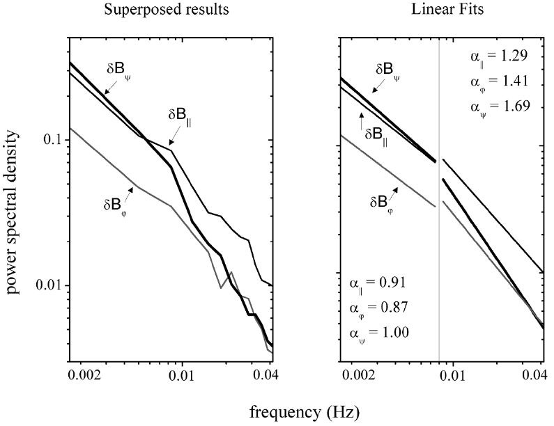
Second, we have superposed the power density profiles of all of the 47 events to obtain average patterns, and this was done separately for each of the three detrended components, the results of which are shown in Fig. 4 (left).

A visual inspection immediately indicates an overall

steeper slope for the ψ component than for the other two, being basically consistent with the conclusion drawn in Fig. 2. Another interesting feature is that for all three components, there is a break frequency near ~0.008 Hz that divides the power profiles into two frequency domains having different slopes. By applying the linear fits to the two domains separately, the spectral indices were obtained, as indicated in the right panel. The spectral indices are largest for the ψ component in both domains. For reference, these are 1.08, 1.11, and 1.47 for α_II, α_φ and α_ψ, respectively, when the fits are done for the entire frequency domain without the division. Thus the largest index value, which is for the ψ component, is larger by >30% than that for the parallel component.

In summary, this paper reports on the determination of power spectral indices for the magnetic field fluctuations associated with magnetic field dipolarizations. For the study, we used the magnetic field data of the THEMIS A, D and E satellites in the near-tail region, identified a total of 47 dipolarization events in February 2008, and performed the FFT power spectral analysis to estimate the spectral indices in the frequency regime from 1.3 mHz to 42 mHz. The obtained values of the indices clearly indicate the existence of anisotropic magnetic turbulence for many events. The degree of the anisotropy as defined by the ratios of the index of the perpendicular components to that of the parallel component can range from ~0.2 to 2.6. There are more events associated with a ratio larger than unity (i.e., the perpendicular index being larger than the parallel index) than those that are anisotropic in the opposite sense. Statistically, the spectral index for the perpendicular direction can be larger by >30% than that for the parallel direction. Also, it is more often the case that the ψ component index is larger than the φ component index in the perpendicular plane.

Our results are preliminary in a few aspects. The most serious defect is our choice of the frequency range, 1.3 mHz to 42 mHz, to apply linear fits. This is similar to what was used in Borovsky et al. (1997). The choice of such a frequency range has something to do with the concept of the so-called inertial range, for which the turbulence structure evolves in a conservative way. The inertial range is bounded by an injection frequency at which turbulence is initially excited, and a dissipation frequency at which the turbulence energy starts to dissipate. However, in the plasma sheet, it is largely unclear at the present time how (and if) one can define an inertial range. Clearly, further in-depth research on this issue is required. For our preliminary study, we have selected this particular frequency range based on the following argument. The injection frequency is taken by assuming that the magnetic turbulence is driven by an excitation on a time scale of 10-15 minutes. This is based on the currently popular view that magnetic dipolarizations are likely caused by the arrival of fast flows, having a time scale of 10-15 minutes in many cases. The dissipation frequency is set by considering proton gyro-frequency in a magnetic field of 25-30 nT. It has frequently been postulated that some kinetic dissipation process likely takes place on a time scale of ion gyro-frequency. Depending on the specific inertial range for which one does fitting to the power spectrum profiles, the spectral index values may differ from what we obtained. Nevertheless, we expect that the main point indicating the ψ?oriented anisotropy will remain valid, though further studies will have to test this when the concept of the inertial range is firmly settled.

Making a direct comparison of the present results with the usual magnetohydrodynamic (MHD) turbulence is not straightforward. One main reason for this is that one needs to convert the frequency spectra into the wave number spectra, and the best approach to this is still unclear. According to Borovsky et al. (1997) and Borovsky & Funsten (2003), a sweeping technique may be used under the Taylor hypothesis to obtain the implication that the spectral indices for the frequency spectra is preserved for the wave number spectra. However, the validity of this argument is not clear for the situations we have dealt with here. Nevertheless, if one is willing to accept the implication based on the argument by Borovsky et al. (1997) and Borovsky & Funsten (2003), a comparison of our results with the standard MHD turbulence theories can be done, as follows.

The homogeneous MHD turbulence theory suggests that the energy spectrum perpendicular to the local magnetic field direction is basically equivalent to the usual Kolmogorov spectrum, the spectral index being given by 5/3, and the parallel spectrum given by the larger spectral index value, 5/2. In contrast, our results indicate that the spectral indices for the perpendicular (parallel) components are often (always) smaller than the homogeneous MHD values. Furthermore, the characteristic anisotropy in the plasma sheet is quite different from, and is statistically opposite to, what the classic homogeneous MHD turbulence predicts. The precise reason for these differences is not currently understood, but they clearly imply that the nature of the turbulence of the usually inhomogeneous plasma sheet can differ significantly from the classic homogeneous MHD turbulence. A larger spectral index for the perpendicular fluctuations than for the parallel fluctuations implies that the fluctuation power decays toward the high frequency regime at a faster rate for the perpendicular fluctuations than for the parallel fluctuations. This could be related to a kinetic mechanism that causes the wave to decay more efficiently at the higher frequency in the plasma sheet. Observational test of this possibility may be worthwhile. We plan to further investigate these issues in the near future.