Two semi-analytic solutions for a perturbed two-body problem known as Lagrange planetary equations (LPE) were compared to a numerical integration of the equation of motion with same perturbation force. To avoid the critical conditions inherited from the configuration of LPE, non-singular orbital elements (EOE) had been introduced. In this study, two types of orbital elements, classical Keplerian orbital elements (COE) and EOE were used for the solution of the LPE. The effectiveness of EOE and the discrepancy between EOE and COE were investigated by using several near critical conditions.The near one revolution, one day, and seven days evolutions of each orbital element described in LPE with COE and EOE were analyzed by comparing it with the directly converted orbital elements from the numerically integrated state vector in Cartesian coordinate. As a result, LPE with EOE has an advantage in long term calculation over LPE with COE in case of relatively small eccentricity.
The motion of the satellite around the Earth can be expressed as a simple Newtonian equation in the Earth centered coordinates. The two bodies rotating around each other without any external forces can be described by the exact mathematical solution. We generally call this simple analytically solvable problem a two-body problem. However, the motion of the satellite in real environment is also dictated by the gravitational and non-gravitational forces due to the irregular shape of the Earth, other celestial bodies, the Earth’s atmosphere, Solar wind, and planetary radiation, etc. These forces other than the point mass gravitational force are called perturbation forces. Even before Classical Dynamics and Mathematics were well defined, some of giants in the science left a big footprint in describing the satellite (planetary)motion with the perturbation (Broucke & Cefola 1972, Taff 1985).
Several methods to calculate the evolution of the satellite’s orbit governed by the perturbation were discovered since the Principia of Newton. The Lagrange and Gauss planetary equations (LPE and GPE) are two most recognized methods to describe the change rates of orbital elements with the partials of the disturbing forces. With these theories, Kozai (1959) and Brouwer & Clemence(1961) derived the semi-analytical solutions for the short period, long period, and secular perturbations with the variety of mathematical techniques.
With the recent development of the modern computer,many of precision orbit propagation tasks have been processed with direct numerical integration (DNI) of the Newtonian equation of motion as the convention of the Cowell’s orbit integration method. The DNI method has achieved one centimeter level of precision orbit propagation (Luthcke et al. 2003). One day arc to even over ten years arc of satellite’s orbit can be propagated by the DNI method to be estimated for the analysis of the perturbations (Nerem et al. 1993). However, the degradation of orbit propagation due to the integration and numerical errors is inevitable as the integration time span grows. Also, the computation time increases as the requested integration time span is getting inflated. To avoid the several inconvenient factors mentioned previously, the analytic or semi-analytic orbit propagators are still investigated and applied in many Celestial Mechanics and Orbital Mechanics problem.
As the development of a domestic satellite orbit propagator and estimator Korea Astronomy and Space Science Institute Orbit propagator and Estimator (KASIOPEA) is right on track (Jo 2008), the characteristic figures of the equations of motion, invariants, and primary variables to be considered must be investigated.
In this study, two types of LPE orbital solutions with classical Keplerian orbital elements (COE) and EOE were reviewed. Before the effectiveness of EOE and the discrepancy between EOE and COE were investigated by using several near critical conditions, a result from DNI had been tested for a reference by the two-body analytic solution. Two types of solution and integration were performed for three different lengths of time. The 13,000 seconds, one day, and seven days evolutions of each orbital element described in LPE were analyzed by comparing it with the directly converted orbital elements from the numerically integrated state vector in Cartesian coordinate.
2. LAGRANGE PLANETARY EQUATION WITH CLASSICAL ORBITAL ELEMENTS
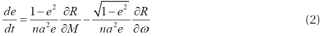
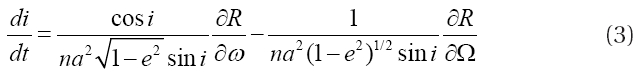
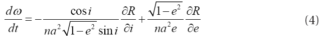
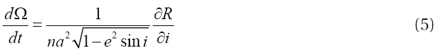
The general theory for finding the rates of change of the osculating elements has been known as the LPE of motion, or simply the Lagrangian variation of parameters (Vallado 2004). In two-body problem it is confirmed that the position and velocity components (in Cartesian coordinates) at any instant permit the determination of a unique set of six COE. And these COE do not change with time. However, most of problems we encountered in the satellite motion have the relatively larger acceleration from the primary body and perturbing accelerations from the others. The equation of the motion of a satellite may be put in a form of Cartesian rectangular coordinates: (
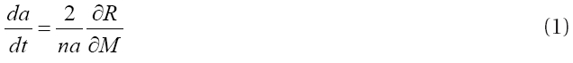
where,
a semi-major axis
e eccentricity of orbit
i inclination of orbital plan
ω argument of perigee
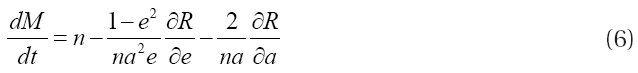
M mean anomaly
Ω ascending node
n mean motion
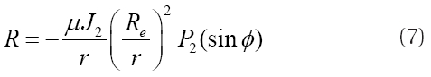
R disturbing function
Using this LPE, we can investigate the perturbation characteristics of specific orbital element with the specific perturbing force. In our case, the time dependent changes of the orbital elements due to the
where,
μ gravitational constant multiplied by
the mass of the Earth
= 3.986004418×10¹⁴ (m3/sec2)
(Vallado 2004)
r radius of satellite
Φ latitude of the sub-satellite point
R2 radius of the Earth
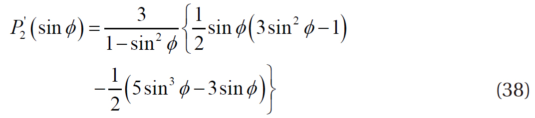
P2 Legendre polynomial degree 2
=2/1(3sin2Φ-1)
However, the disturbing function,
where,
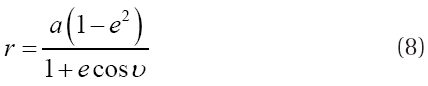
υ true anomaly
With the perturbation by the
3. LAGRANGE PLANETARY EQUATION WITH EQUINOCTIAL ORBITAL ELEMENTS54
With the COE in LPE, there can be some inconvenience with specific types of orbits. As you can see in Eqs. (2-6), small eccentricities or small inclinations can make the equation unstable. The eccentricity and the
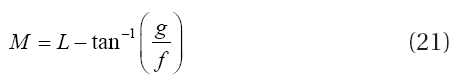
The transformation from the equinoctial elements to the COE is given in Eqs. (16-21).
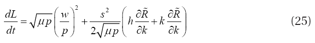
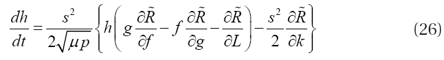
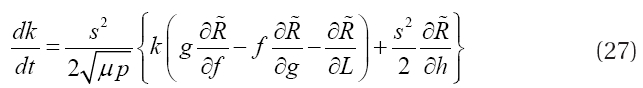
With the calculation of Lagrange bracket with the EOE and the differentiation of Eqs. (10-15) with respect to time, the derivatives of EOE can be found in terms of COE and their derivatives. Eqs. (1-6) can be replaced by the new set of LPE, Eqs. (22-27).
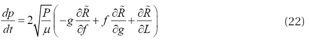
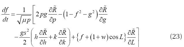
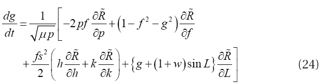
where

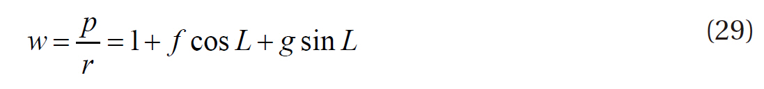
The disturbing function, Eq. (7) can be rewritten with the substitution of Eqs. (30) and (31).
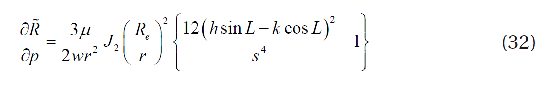
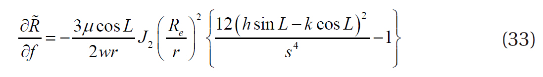
New set of derivatives of the disturbing functions in terms of EOE is shown in Eqs. (32-37).
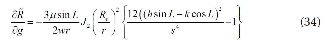
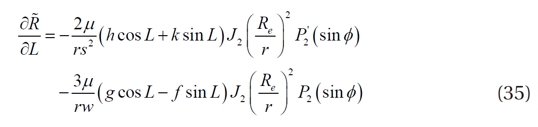
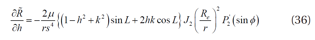
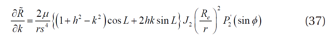
where
The description of the orbit evolution by the
4. DIRECT NUMERICAL INTEGRATION OF THE EQUATION OF MOTION IN CARTESIAN COORDINATE
A state vector and a force vector in Cartesian coordinate can be defined as in Eqs. (39) and (40)
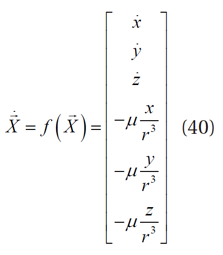
where
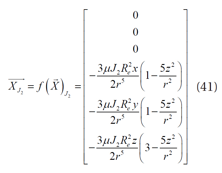
The acceleration due to the
where,
The equation of motion expressed in the Cartesian coordinate has an advantage in the numerical integration for its simplicity over analytic or semi-analytic type. And the perturbation functions and two-body equations do not have any singular point except
The transformation from the state vector to the COE can be achieved without any trouble in most elliptic case. The full procedure for this transformation can be found at Vallado (2004) and other references. Unlike semi-analytical solutions, this DNI method may introduce an error as time increases: truncation error. This type of error cannot be avoidable as the computer has limited digit of significant number and the numerical integration method inherits the approximation errors.
In this study, the comparison of the results from the each solving method of the equation of satellite motion with
First, four specific orbits chosen to represent particular orbit might introduce some inconvenience. The case I in the Table 1 represents an orbit with very small eccentricity and small
Second, the accuracy of the numerical integration of the equation of the motion with two-body force only in Cartesian coordinate was compared with the analytical
[Table 1.] Initial condition (Keplerian elements).
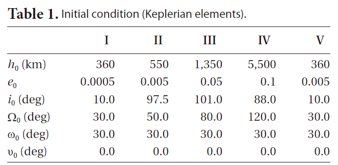
Initial condition (Keplerian elements).
solution: mean motion on the orbital plane. To validate the DNI method, all cases of initial condition were tested. The value of
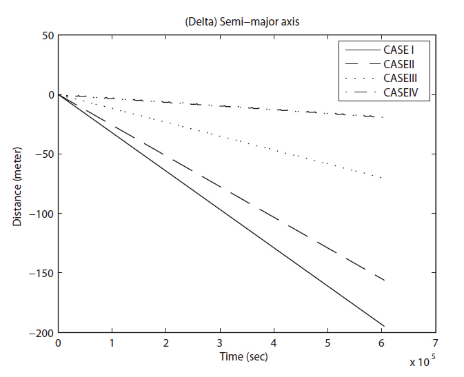
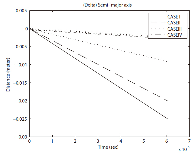
The difference (error) evolutions of orbital elements between the DNI method and the analytical solution are shown in Figs. 1-7. In case of DNI method, the integration time step must be chosen with careful consideration for classical Rung-Kutta 4th order method to minimize calculation load, round-off error, and truncation error. However, it is not a simple task to find an optimal integration step size for general cases.
In this study, fixed step sizes: 60 and 10 seconds were tested for all cases. As shown in Figs. 1 and 2, the accuracy was improved in 1 to 1,000 ratio as the time step was reduced in 6 to 1 ratio. With the integration step size of 60 seconds, error in the semi-major axis grows to about 200 meters for the case IV in 7 days. With the integration step size of 10 seconds, same orbit has only 0.025 meter error after 7 days. An optimal integration step size can be found with further test or an integration step size control can be applied to this study. However, 10 second step size was chosen for its obvious simplicity in decimal number with relatively acceptable accuracy.
The error in semi-major axis grows almost linearly as time advances for all four cases as shown in Fig. 2. The shorter period the orbit has (i.e. the orbit is closer to the
Earth), the steeper slope the error shows. Since we used a fixed size integration step for all numerical integrations, the orbit with larger orbital period requires larger number of integration step to complete one revolution. It has benefits of smoother and dense derivatives, and shorter interval relative to the whole arc of orbit. Unlike other cases, the case IV shows the sinusoidal behavior with same period of orbital revolution
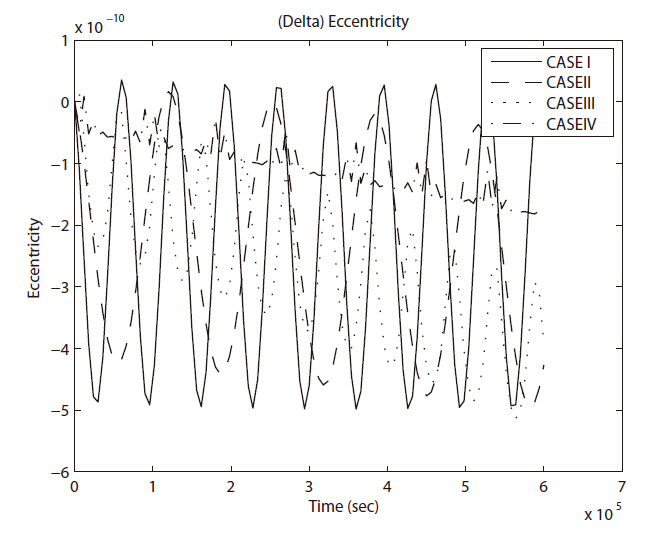
More complicated figures are shown in the error evolution in eccentricity for all cases as you can see in Fig. 3. The sinusoidal variation of each case shows same periodicity of orbital revolution. Over all tendencies are similar to those in semi-major axis case. However, the eccentricity looks more susceptible to the errors induced by the numerical integration.
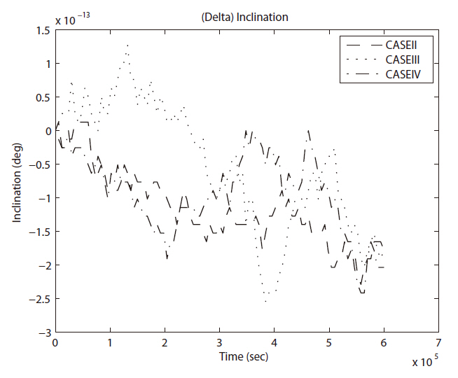
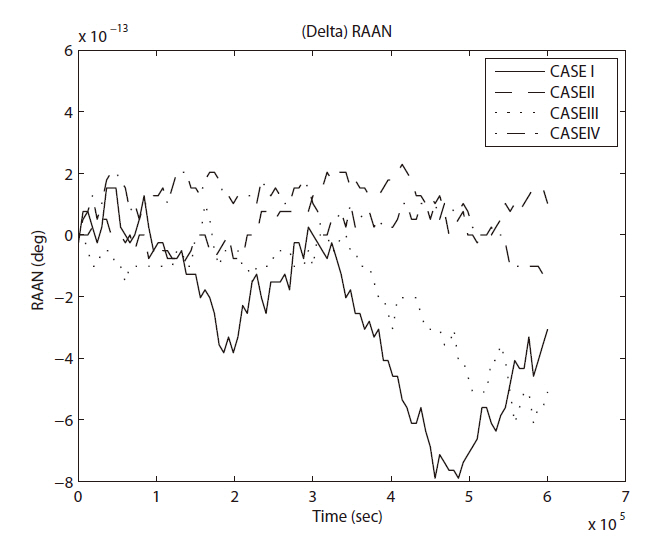
The error evolutions of inclination and the right ascension of ascending node are shown in Figs. 4 and 7 respectively. In these two cases, it is hard to find any periodicity or obvious tendency except gradual degradation. The magnitude of the errors in both cases lies close to the lower bound of significant number of digit of the computer used in this study compare to the original values of both orbital elements.
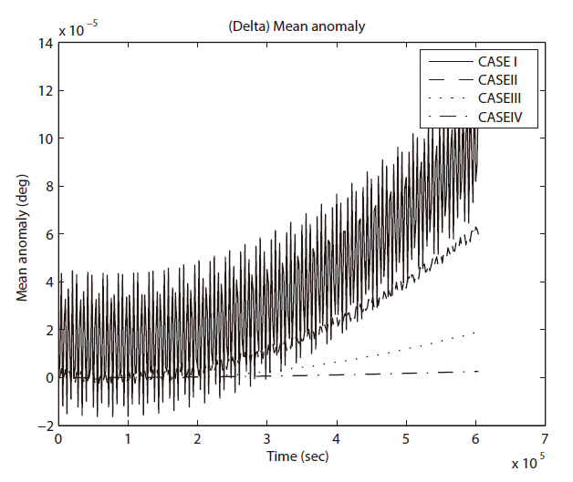
The fast variable in the LPE, mean anomaly shows typical error evolution figures in Fig. 5. As shown in Fig. 6, the effect of error on the argument of perigee is stronger as shallower the ellipse is.
In summary, the deviations of the DNI method from the exact solution for two-body problem do not exceed 10-6 ratio in case of
Third, the general perturbation solutions by using COE and EOE shown in Appendix A and B are calculated and the set of state variable with
6. COMPARISON RESULTS AND DISCUSSION
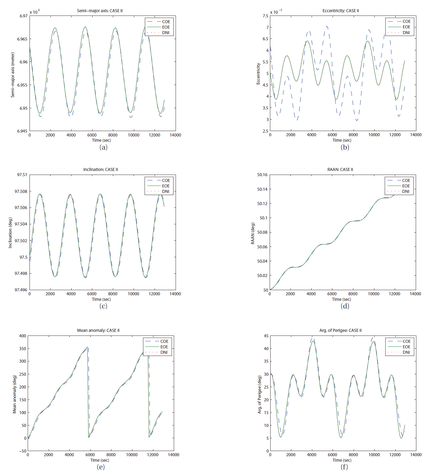
The time evolution of each orbital element (whether it is integral or variable) by three different approach for solution was investigated with the initial conditions suggested in the previous section. The initial condition of orbits to be investigated was chosen to check the system instability caused by the near singular condition in the denominators of the equations.
The first comparison test with 13,000 seconds duration, which represents one revolution of the longest period of test orbit (case IV), is expected to show major characteristics of short period perturbation as
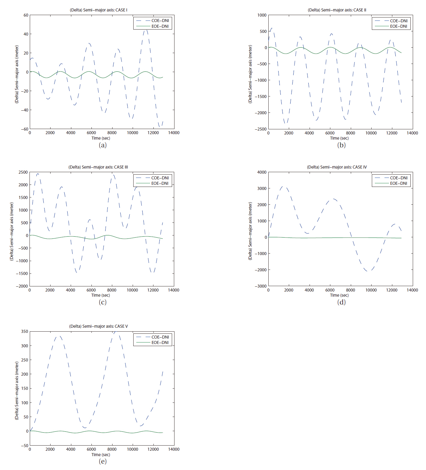
The difference evolution in semi-major axes of two semi-analytic solutions from the DNI result is shown in Fig. 9. The gaps at the epoch (t = 0) in Fig. 9 were produced by the off-set due to an addition of first solution from the LPE with COE. Even application of mean value to adjust osculating orbital elements to mean orbital elements (Not mean orbit) cannot get rid of these gaps completely. The arbitrary initial orbit elements as shown in Table 1 are used for orbit simulation in this study, however, we obtain an osculating orbital element from the calculation of the Lagrange planetary equation’s solution with perturbing forces. The result from LPE with perturbing forces is always an osculating orbit. In other words, using a priori orbit elements, perturbed orbit must not be admitted to use at next epoch. This can be adopted both COE and EOE case. In the DNI case, a numerical integration of dynamics including perturbations produces an osculating orbit at any epoch naturally.
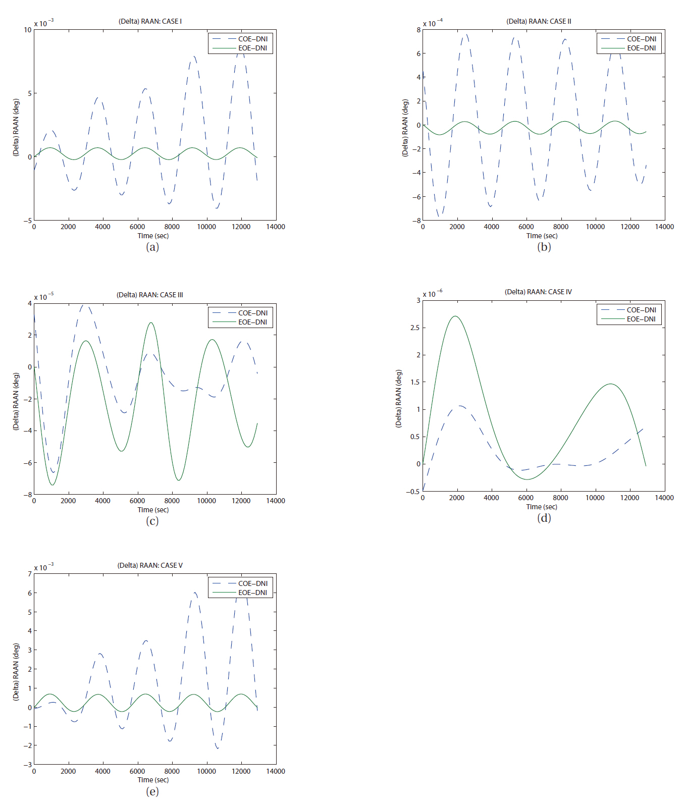
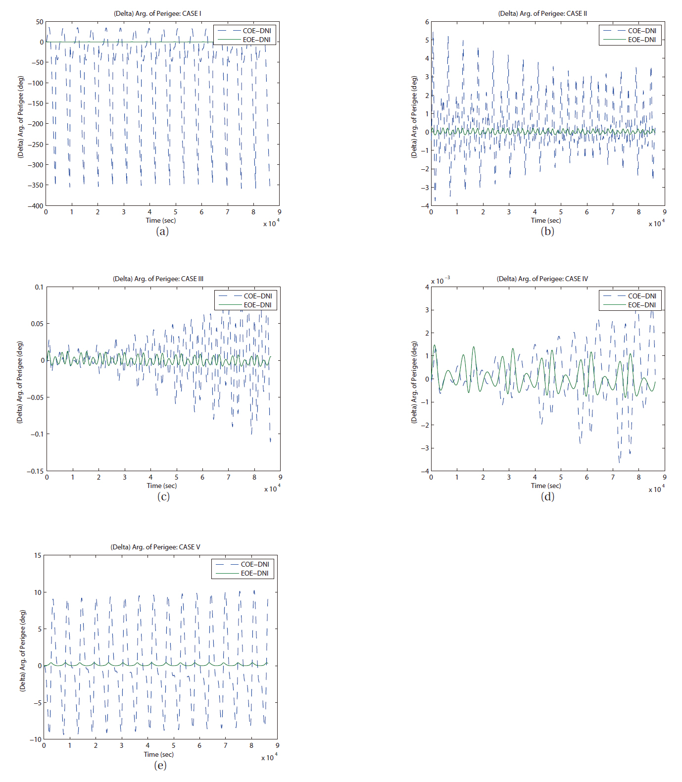
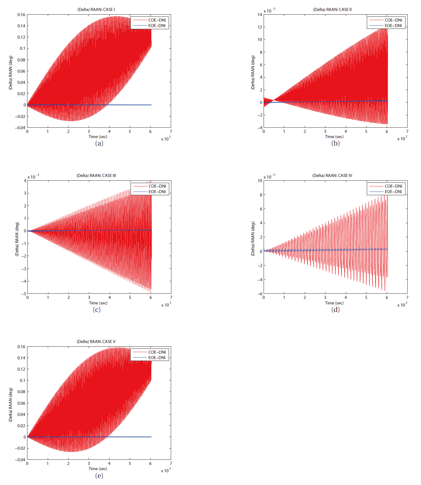
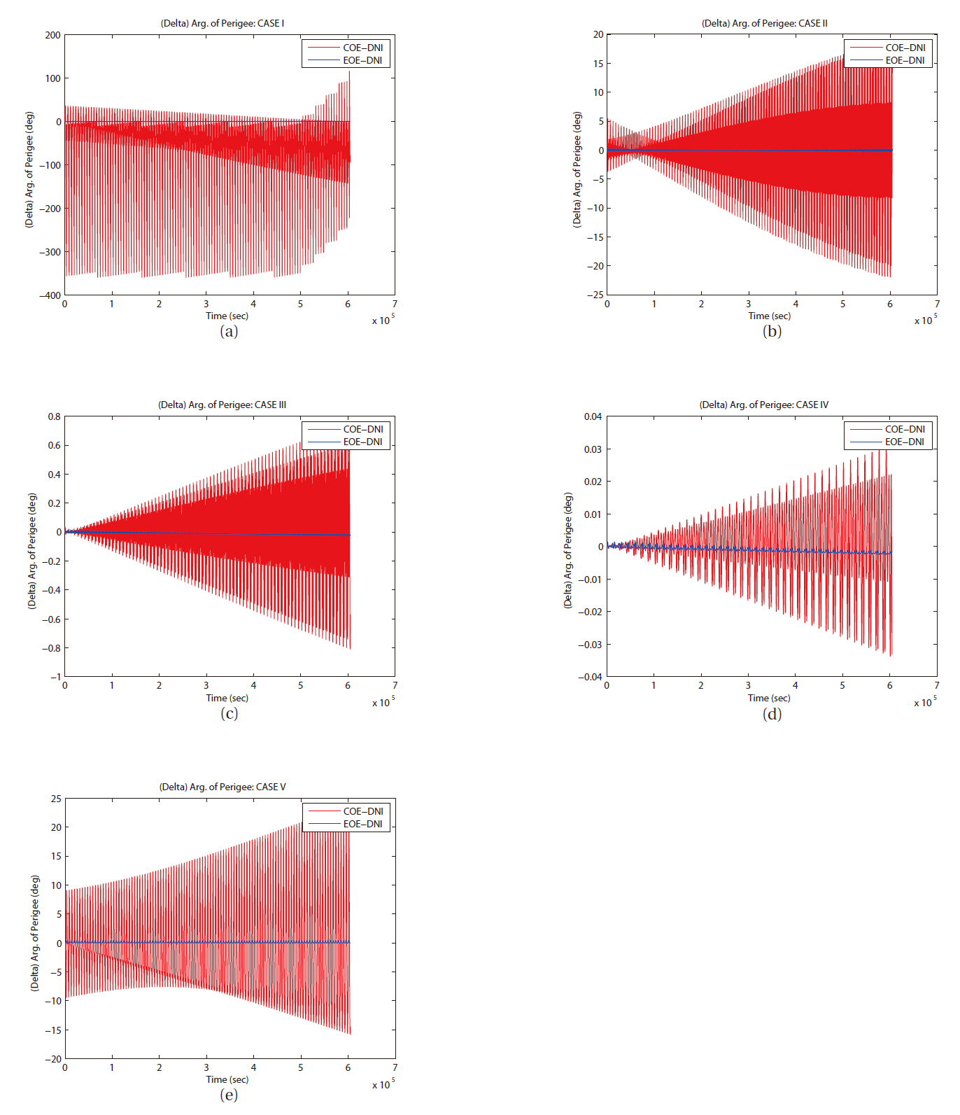
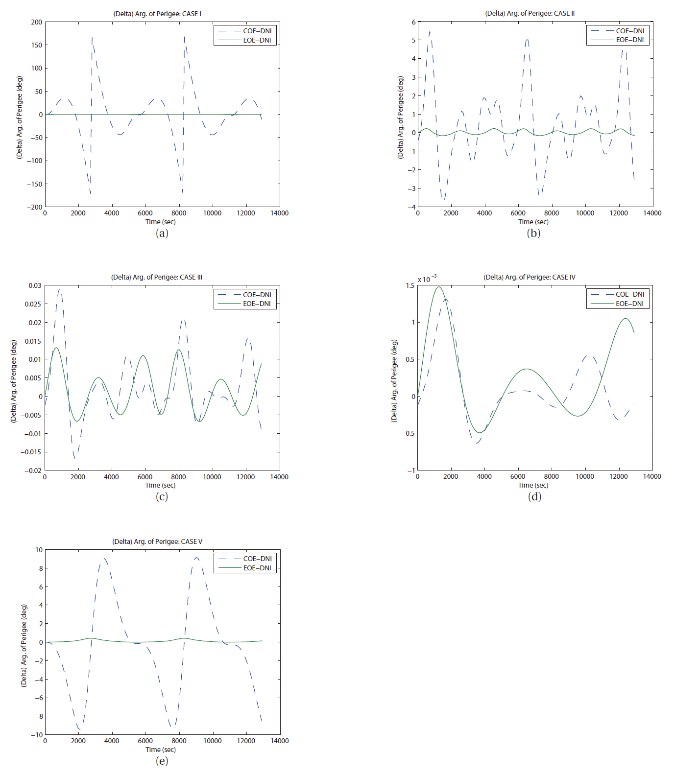
As we have mentioned, LPE uses input elements as a reference orbit and calculates each element’s variation caused by perturbations. In this study, orbit simulation of each case has been set a same initial condition, so same orbit elements can be used as an initial value for input at each case, COE, EOE, and DNI. The difference evolution of right ascension of ascending node for all cases is shown in Fig. 10. The inclination and the ascending node decide the spatial position of an orbital plane in an inertial frame. The trends of the evolutions of the inclination and the right ascension of ascending node are very similar naturally. As shown in Fig. 11a, the amplitude of error variation in argument of perigee is relatively larger than any other angle related orbital elements. However, the error of mean anomaly in the case I by COE LPE shows unreasonable behavior compared to the results from other method. For the analysis of this type of error in the case I,
the initial condition of the case V was selected. The initial condition of both cases has identical components except eccentricity. The eccentricity of the case V is exactly ten times of that of the case I. As the eccentricity in the case I was 0.0005, both terms in the right hand side of Eq. (2) induced some inconveniency. On the contrary, the one in the case V with the value of 0.005 did not introduce same magnitude of troubles. More rigorous analysis on the evolution of the eccentricity will be performed on a separate study.
The second comparison test was performed in same manner with one day duration to check the consistencies.Also, we can check the slight hint of long term error behavior of each orbital element from different solutions.
With the seven day duration of time, only few details of variation trend can survive.
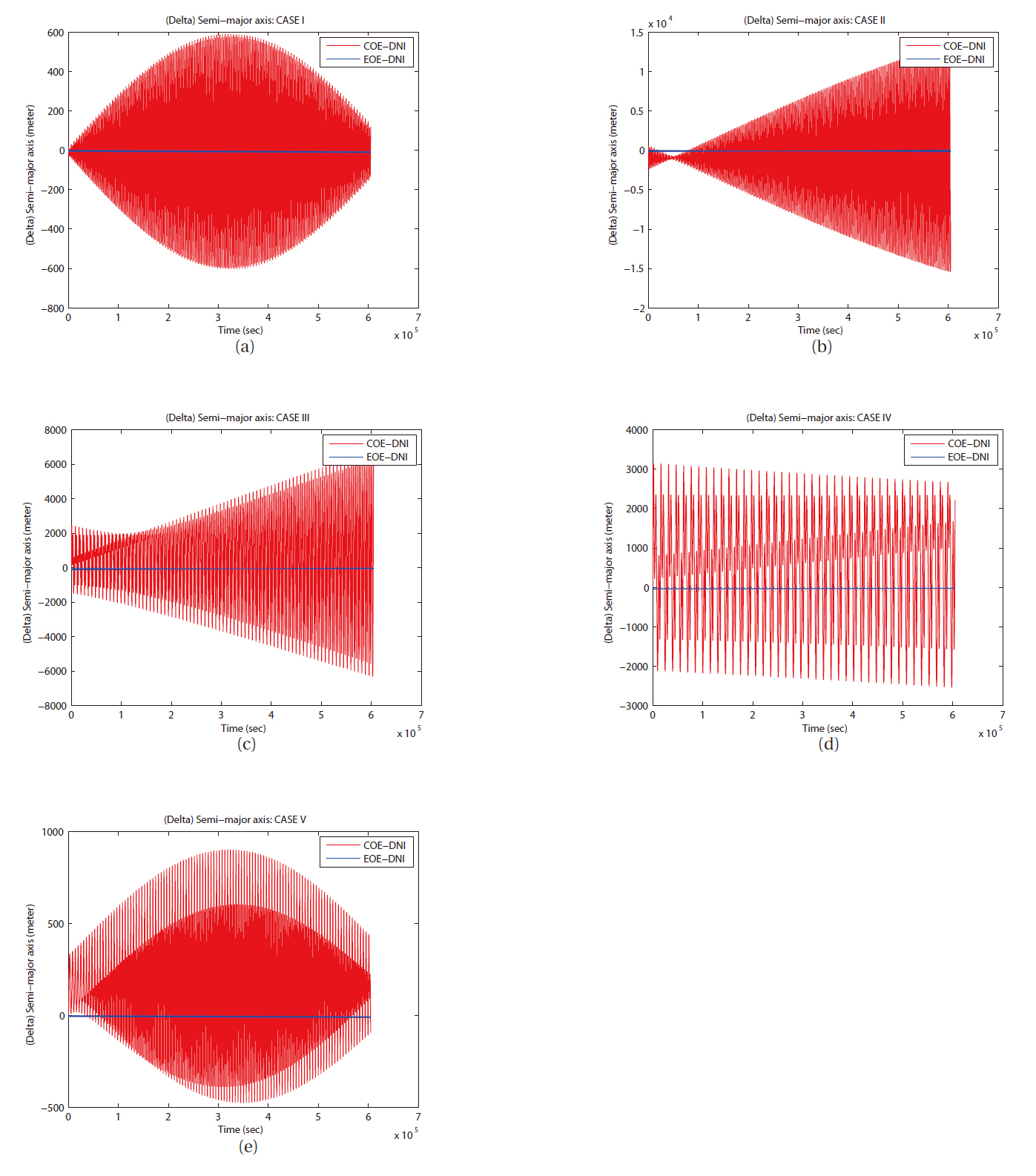
In Fig. 12,you can find the various types of error evolutions of semi-major axis. With only J2 perturbation, long period perturbation behavior was not expected. The orbital trajectory from each method (LPE with COE, LPE with EOE, and DNI) did not show obvious long periodic perturbed motion in seven days. However, the cases I, II, and V show periodic variation in errors semi-major axis as shown in Figs. 12a, b, and e. Also, you can see similar variation in right ascension of ascending node as in Figs 13a-c, and e. In case of argument of perigee, same kind of periodic variations can be seen in Figs. 14b and c. But it cannot be confirmed as a long period perturbation with-
out further analysis.
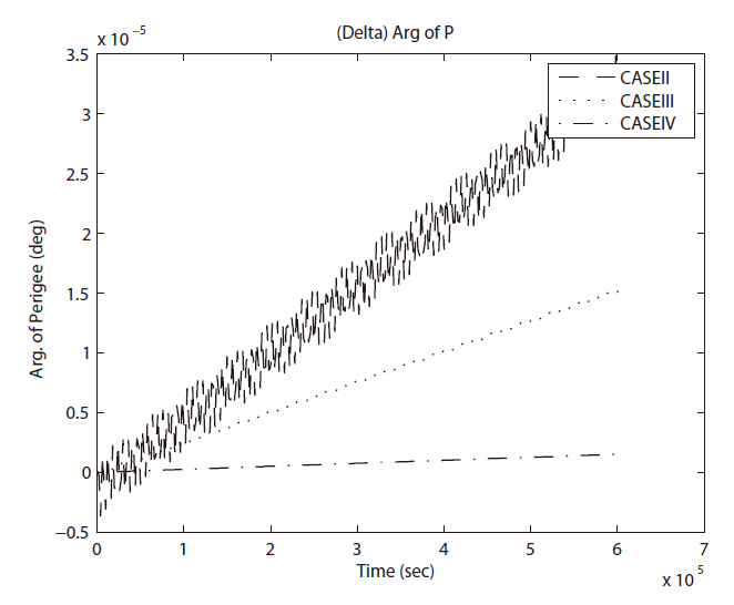
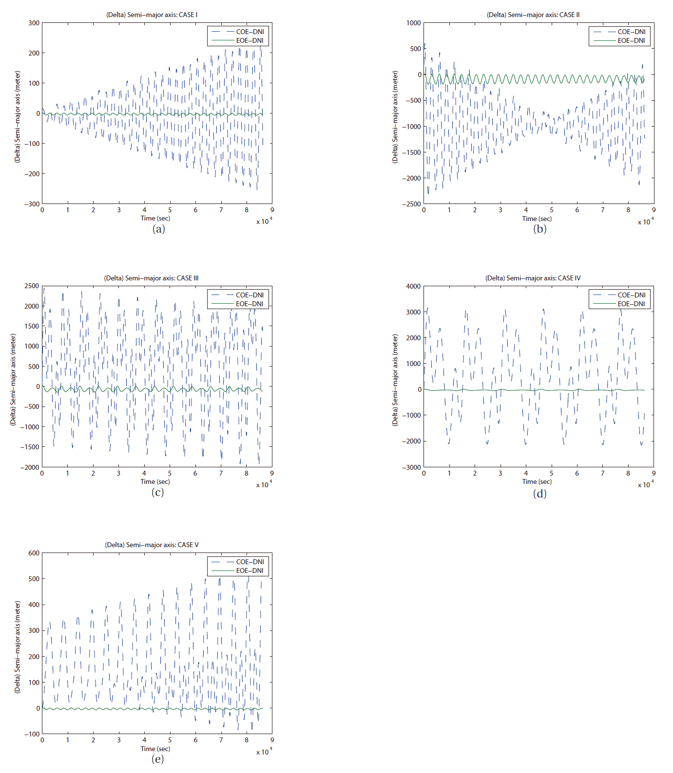
Then the third comparison test was performed in same manner with seven day duration to check the long term variation in each element. With the seven day duration of time, only few details of variation trend can survive. However, the cases I and V show periodic variation in error evolutions in semi-major axis and right ascension of ascending node as shown in Figs. 15a and e, 16a and e. Also, you can see secular like variation in semi-major axis as in Fig.15 d. The divergence trend can be seen in the error evolutions in semi-major axis as in Figs. 15b and c, in right ascension of ascending node as in Figs. 16b-d, in argument of perigee as in Figs. 17b-d.
In summary, the description of a perturbed motion
of satellite by LPE with COE can be erratic on several orbital elements in specific cases like small eccentricity or small inclination. As you can see in most figures, EOE LPE agrees relatively better with DNI method than COE LPE does in most elements. It is consistent with different sizes (semi-major axis), shapes (eccentricity), and orbital plane position (inclination and right ascension of ascending node).
In this paper, we selected only three elements, semi-major axis, right ascension of ascending node, and argument of perigee to present the error evolution by time. However, the position of a satellite on an orbit can be defined by mean anomaly. This non geometric angle plays an important role as a running variable instead of time
in LPE with COE. In this study, the trends of variation in mean anomaly for each case shows similar pattern as in argument of perigee. In the same manner, (semi-major axis, eccentricity), (right ascension of ascending node, inclination), and (argument of perigee, mean anomaly) can be loosely couple by its similarity in the variations.
The theories and equations we used in this study are consistent with Kozai (1959), Brouwer & Clemence (1961) and Vallado (2004). And the result from EOE LPE and DNI agreed each other. Not until further study and analysis are performed, the long periodic variations in the solutions of COE LPE cannot be confirmed.
In this study, we compared the three methods to describe the motion of a satellite with the
A. Short periodic perturbation on orbital elements by
[Table A1.] Initial condition in Cartesian coordinate.
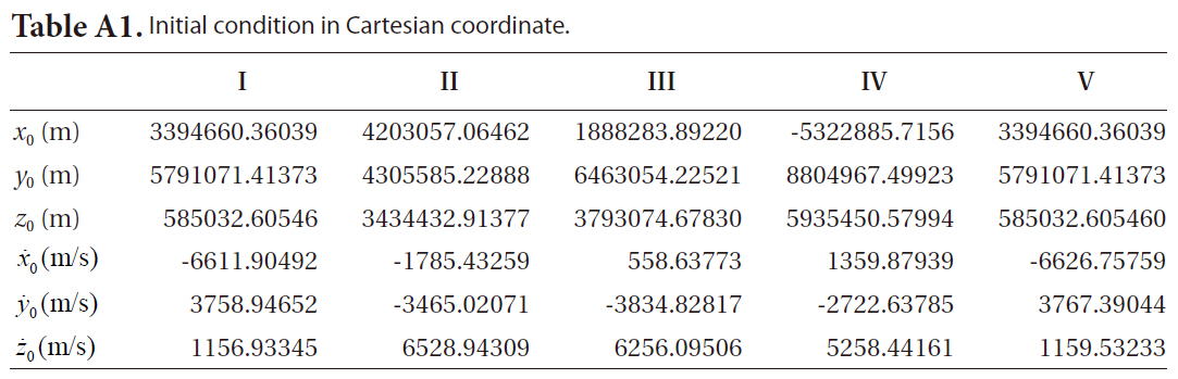
Initial condition in Cartesian coordinate.
B. Secular perturbation on orbital elements by the