In general, inertia properties of a spacecraft are measured before the launching and they are used in controlling the attitude for the spacecraft to perform its mission.However, ??the inertia properties are changed when situation that may affect the mass of the spacecraft occurs such as the decrease of the mass of the spacecraft by the consumption of propellant during the mission implementation.Moreover, when the mission requires detailed control of attitude, precise estimation of the inertia properties is necessary since change of them may have a great influence on the attitude control.
The attitude information of the spacecraft is used in estimating the inertia properties and the information includes noise. Since the inertia properties estimation by least squares method is susceptible to noise, noise-effect should be firstly reduced. To avoid such a procedure, an inertia properties estimation method based on the law of conservation of angular momentum was suggested and applied to actual estimation of inertia properties of a spacecraft (Peck 2000, Lee & Wertz 2002). This method was studied for the cases where only one axis is maneuvered and where the moment of inertia is very large when compared to the product of inertia. One of drawbacks of this method is that the estimation error of the inertia is very large when all the three axes are maneuvered simultaneously.However, since it is impossible to maneuver only one axis when there exists product of inertia, the maneuver of three axes should be considered. In addition,accurate estimation of the product of inertia is necessary for the case of precise control.
In this paper, a modified method for inertia properties estimation based on the law of conservation of angular momentum is proposed for the case when three axes are maneuvered simultaneously. The process to reduce the estimation error in the product of inertia is shown and the performance is verified by comparing the inertia properties estimation based on least squares method and the law of conservation of angular momentum as well as the proposed method.
2. INERTIA PROPERTIES ESTIMATION TECHNIQUE
2.1 Inertia estimation based on least squares method
The equation of motion including the control input by reaction wheels can be expressed as Eq. (1) (Hughes 1986):


where
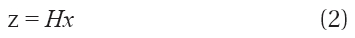
For the inertia properties estimation based on least squares method, the equation is rearranged as Eq. (2):
where
Using least squares method, the estimated value

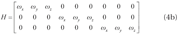
Here, the elements of the matrix, H, are the information including noise. A rank of the matrix should be the maximum and the measured vector,
The variables in Eq. (3) are expressed as Eq. (4):


Here, the estimated value
2.2 Inertia estimation based on the law of conservation of angular momentum
When a spacecraft is maneuvered using reaction wheels, all the angular momentum of the spacecraft is conserved in the inertial frame under the assumption that the disturbance is very small.
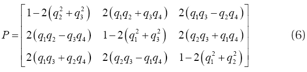
Defining
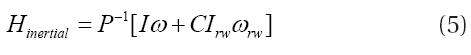
Here, the transformation matrix
According to the law of conservation of angular momentum, Eq. (7) is valid since the angular momentum should remain constant before and after the spacecraft maneuvering.

Assuming the initial angular velocity of the spacecraft to be 0, the
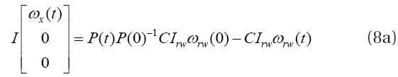
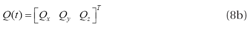
Defining the right side of the Eq. (8a) as Eq. (8b) and inputting this in the Eq. (8a) again, Eq. (9) is derived by considering the first element:
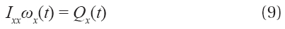
The estimated value I
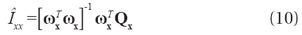
Here, ωx and Qx are N by 1 column vectors. Repetition of the above method using [ωx, Qy],[ωx, Qz] gives the estimated values
2.3 Inertia estimation based on modified law of conservation of angular momentum
The inertia properties estimation method based on modified law of conservation of angular momentum is proposed to make it possible to estimate inertia properties in the case when three axes are maneuvered and to improve the accuracy of the product of inertia estimation.
Assuming that the angular momentum is constant before and after the spacecraft maneuvering, Eq. (7) can be arranged as follows:
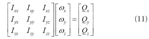
Rewriting of the first row of Eq. (11) gives Eq. (12):
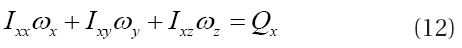
Since the moment of inertia,
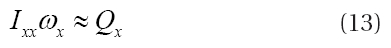
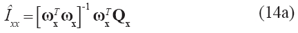
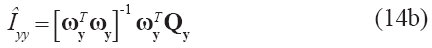
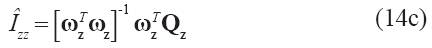
By expressing the second and third row of Eq. (11) in the same manner shown above, the moment of inertia with respect to each axis can be estimated as in Eq. (14):
The moment of inertia estimated by the procedure shown above is used for the calculation of the product of inertia as shown in Eq. (15):

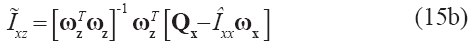
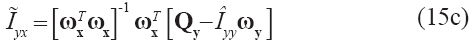
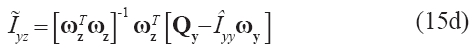
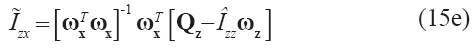
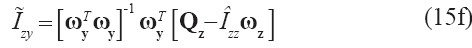
Eq. (15) indicates that the calculation for the estimation of the product of inertia is carried out using only the estimated moment of inertia. For example, in the procedure of calculating
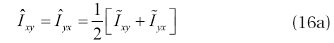
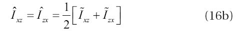
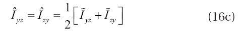
The pair of product of inertia estimated in the same conventional method is averaged for the calculation as follows:
3. SIMULATION RESULTS AND ANALYSIS
For the comparison of the inertia properties estimation methods mentioned above, a numerical simulation is performed. The simulation parameters are listed in Table 1.
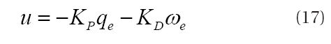
The controller in Eq. (17) is used for the attitude control.
[Table 1.] Simulation parameters.
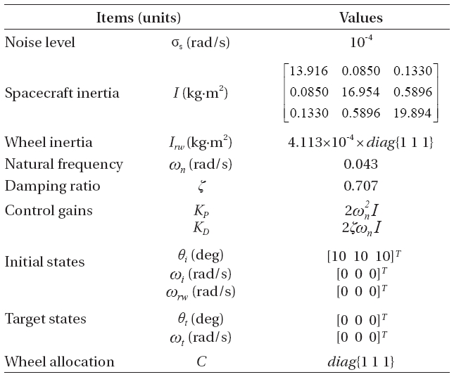
Simulation parameters.
where
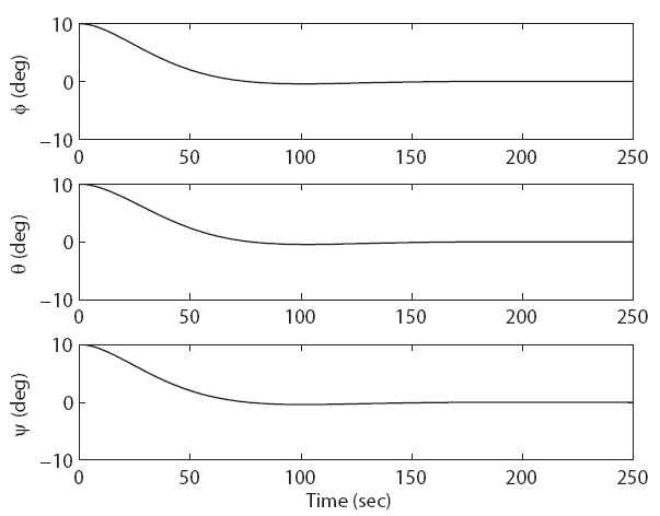
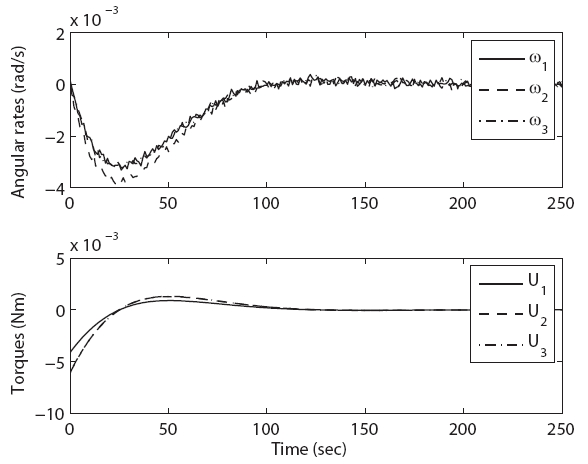
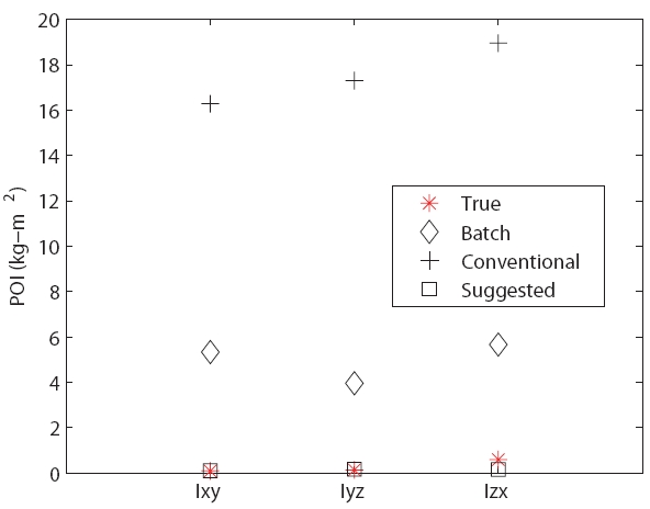
The angle, the angular velocity of the spacecraft, and the control input from the numerical simulation are shown in Figs. 1 and 2. Based on these data, the inertia properties are estimated by the methods mentioned above and the results are shown in Table. 2 and 3, and Figs. 3 and 4, respectively.
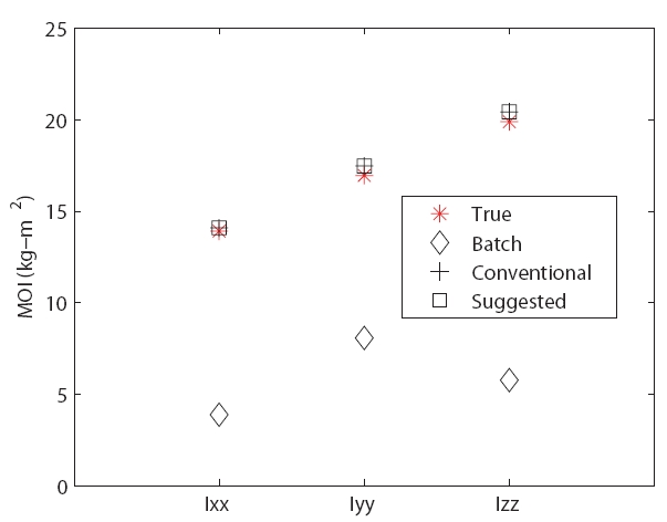
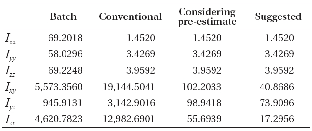
In Table 2, “True” indicates the actual inertia properties of the spacecraft, “Batch” the values estimated by using least squares method, “Conventional” the values estimated by using the conventional method based on the law of conservation of angular momentum, “Considering pre-estimate” the estimated values obtained by using the previously calculated product of inertia in the calculation of the next product of inertia, and “Suggested” the values estimated by using the method that the author propose.
[Table 2.] Estimation results (kg·m2).
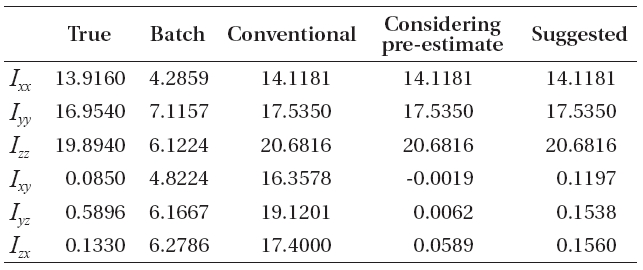
Estimation results (kg·m2).
[Table 3.] Comparison of the errors (%).

Comparison of the errors (%).
Quite large errors are found between the estimated values and the actual inertia properties in the case where least squares method is used. When this method is applied, nine inertia properties are calculated at once as shown in Eqs. (3) and (4). However, as described in Section 2.3, least squares method is individually applied for the calculation of the nine individual inertia properties when the law of conservation of angular momentum is used. For example, in the process of calculating
In the case when the conventional method based on the law of conservation of angular momentum is used, the moment of inertia is well estimated, but the error is very large in the product of inertia. This is because, when all the three axes are maneuvered, the maneuvering of the other two axes is not considered.
The proposed method shows the same error in the estimated moment of inertia with that of the conventional method based on the law of conservation of angular momentum. However, relatively better results are obtained in the product of inertia when compared with the two methods mentioned previously. As noted in Section 2.3, in the calculation of product of inertia, less error is found when the product of inertia calculated in advance is not used in the estimation of the product of inertia. In addition, among the product of inertia estimated by the proposed method,
The study in this paper is conducted by focusing on the following three aspects: first, simultaneous maneuvering of three axes is considered since maneuvering of only one axis is not possible where there exists product of inertia; second, when using the attitude information including noise, the conventional attitude information is used without the noise-effect compensation procedure using filters; finally, an accurate method for the estimation of product of inertia is proposed, which showed far better result than that of the conventional methods.
In this study, inertia properties are estimated by one time of calculation. In the future study, convergence of the estimated values will be verified by using iteration technique.