The traditional approach to inverting aerosol extinction makes use of the assumption of a constant LIDAR ratio in the entire Mie-LIDAR signal profile using the Fernald method. For the large uncertainty in the cloud optical depth caused by the assumed constant LIDAR ratio, an not negligible error of the retrieved aerosol extinction below the cloud will be caused in the backward integration of the Fernald method. A new algorithm to determine aerosol extinction below a cirrus cloud from Mie-LIDAR signals,based on a new cloud boundary detection method and a Mie-LIDAR signal modification method, combined with the backward integration of the Fernald method is developed. The result shows that the cloud boundary detection method is reliable, and the aerosol extinction below the cirrus cloud found by inverting from the modified signal is more efficacious than the one from the measured signal including the cloud-layer.The error due to modification is less than 10% taken in our present example.
Aerosol and cloud play a very important role in the earth-atmosphere radiation budget, and they have been considered to be the largest uncertainty in climate change research [IPCC2007]. Extensive observations of aerosol and cloud with active and passive remote sensors have been undertaken worldwide. Taking the advantage of the active optical remote sensing, LIDAR can provide profiles of extinction,their temporal variation, and the depolarization ratio that can be used to estimate the physical state of cloud and aerosol particles and to distinguish them. Except in the case of strong attenuation features (such as low thick clouds and rains), Mie scattering LIDAR can continuously and automatically monitor in real time the particles above the observation sites. These long-term observational data are very useful for studying the temporal and spatial variations of aerosols and clouds and their interactions. So, this kind of LIDAR is widely used for studying aerosol and cloud optical properties in the Anhui Institute of Optics and Fine Mechanics (AIOFM) [1-3], the National Institute for Environmental Studies (NIES) [4] and the National Aeronautics and Space Administration (NASA) [5] as ground-based observations and space-borne measurements such as LITE,GLAS [6] and CALIPSO [7].
In analysis of such LIDAR data, the Fernald [8] and/or Klett [9] methods are often considered to inverting optical properties of floating particles based on an important assumption of a constant relationship between backscatter and extinction. That constant is the extinction to backscatter ratio or LIDAR ratio (
In this paper, a new algorithm to determine aerosol extinction below a cirrus cloud from Mie-LIDAR signals is developed, for which a new cloud boundary detection method and a Mie-LIDAR signal modification method are included together with the backward integration of the Fernald method. Here, the cloud boundary detection algorithm is based on high temporal resolution of the cloud,and a simulated signal is used to substitute the detected cloud-layer signal in the Mie-LIDAR signal modification method. Both of them are generally described in Section II. The application is shown and discussed in Section III,which is followed by the conclusions.
Cloud boundary detection algorithm for a LIDAR signal is an old topic. Several methods have been developed for detecting the cloud boundaries from LIDAR data [13-19],these methods are mainly based on the characters of the LIDAR signal and the physical signature of the cloud.Because of the complexity of the cloud and the different LIDAR configurations, it is very difficult to develop universal cloud boundary detection algorithms for LIDAR use. Most techniques used for cloud boundary detection search for zero crossings in the derivation of the returned signal (the differential zero-crossing method [13]). Others look for a“threshold” value of signal shift from the background (the threshold method [15]) or construct LIDAR clear-sky power return profiles from archived data to test for the presence of clouds (a quantitative approach based on the clear-air scattering assumption [14]). This method avoids some of these problems but is most useful in the upper troposphere,where aerosol returns are generally negligible.. Also, an alternative cloud detection algorithm for optically thin clouds is used in [16]; the algorithms for the detection of hydrometer returns in MPL(micro pulse LIDAR) data are developed by authors in [17]; and a more general cloud detection method which can differentiate among various targets such as clouds, virga, and aerosols to separate cloud from noise and aerosol signals is developed, [19]. Of course, noise estimates and/or smoothing are carefully used in some of those techniques to reject false peaks resulting from cloud inhomogeneity, aerosols and signal noise. But all of those mentioned above are considered the spatial changes of LIDAR signals among various targets such as clouds and aerosols. In this paper, we find a new cloud detection algorithm to separate cloud from noise and aerosol signals, based on high temporal resolution of observations.
The cloud boundaries detection algorithm for Mie scattering LIDAR introduced here, is enhanced by advantages of LIDAR itself, i.e., the high spatio-temporal resolution information of aerosol and cloud can be recorded by it.The information responding to the physical property of cloud and aerosol are considered in the algorithm. Also some thresholds are selected to use for data quality and cloud finding. The algorithm includes three steps:
The first step is to do some preparation. The Mie-LIDAR not only recorded one averaged profile (e.g. by 1000shots)but also each detailed profile (e.g. by 100shots) in a small time interval. For each detailed profile, the measured Mie signal
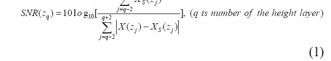
In the algorithm, a maximum effective detecting height
The second step is to record all the possible layers and their boundaries. Examine the σ
The third step is to distinguish the cloud from aerosol layer.The differences of LIDAR signal and physical properties of the cloud and aerosol layer are used to distinguish them. The ratio σ
The algorithm was applied to the data measured using a polarization-Mie LIDAR (PML) [20]; the detected cloud region was validated by depolarization ratio (DR) δ measured synchronously using the same LIDAR. The validation showed that the cloud boundaries could be detected well from the Mie scattering LIDAR data using this algorithm (Section III in this paper).
2.2 Mie-LIDAR signal modification
A Mie-LIDAR signal for a cloud-layer contains information about the aerosol and cloud. As mentioned above, the cloud layer should be eliminated from the LIDAR signal before further analysis. Fortunately, the cloud edges are screened out and their corresponding heights are recorded in the forgoing algorithm. Next, a signal modification algorithm will be presented.
Let us consider the case, in which only one cirrus cloud layer is included in the LIDAR signal and the heights of cloud base and cloud top are marked with
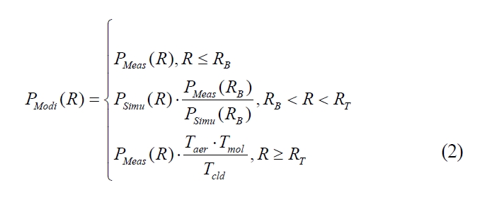
where,
From Eq. (2), the measured LIDAR signal over the range of cloud layer is replaced by a simulated signal at the same range in sliding scale, and the one above the cloud layer is corrected by multiplying the transmittance of the simulated atmosphere layer and dividing the transmittance of the detected cloud layer. Then a modified Mie-LIDAR signal is performed and can be analyzed further.From the LIDAR equation, the aerosol extinction can be retrieved by the traditional Fernald inversion method using the modified signal. For the detected cloud layer, the cloud extinction coefficient can also be derived from transmittance of it by Chen’s method [11].
3.1. Cloud detection and validation
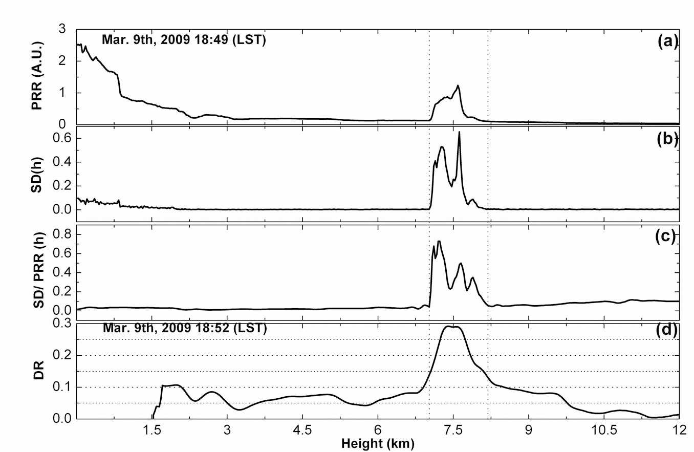
One example of cloud-layer edge detection algorithm is shown in figure 1. The data was measured by PML over Hefei on Mar. 9th, 2009. As mentioned in [3] and [20] PML is a 532 nm ground-based and calibrated polarization Mie LIDAR, which has two Mie scattering detection channels and two alternative polarized detecting channels according to different aims. And the LIDAR specifications are also stated in reference [20]. The PML can get either backscattering information in the entire troposphere or depolarization information above gated-control height as shown in figure 1(a) and figure 1 (d). From the averaged profile of PRR,there are two kinds of particle layers: one is cloud layer at about 7.5 km; the other is an aerosol layer below 3 km.Using the threshold criterion ( σ
possible layers. And the height of the cloud layer is 7.02 km~8.22 km with a peak height 7.59 km. The mean value of
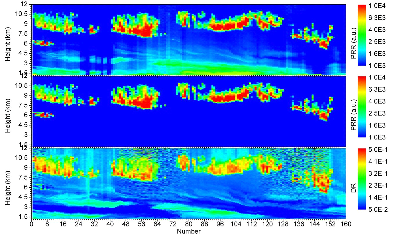
To further testify to the practicality and reliability of this cloud detection algorithm, it was applied to the PML data measured from 16:00 Apr. 2nd, 2010 local standard time (LST) to 21:00 Apr. 4th, 2010 LST with 30 m vertical resolution. The measurement was taken every 20 minutes as shown in Figure 2. In each observation, 2000 laser pulses were fired with a repetition of 10 Hz to get one averaged profile, and each 20s-averaged profile prepared for cloud detection was also saved as one of the time-series profiles. The range-square corrected LIDAR received power, detected cloud boundaries using the algorithm introduced above,and DR of cloud and aerosol are shown in Figure 2. The cloud lies in the range from 5 km to 11 km above the ground level and sometimes the multi-layer cloud is shown in a same profile. Although the geometric depths of some cloud layers are more than 3 km, the laser can penetrate them
because they are high-level cirrus clouds and are mainly composed of ice-crystal particles, which can cause strong depolarization of backscatter light with
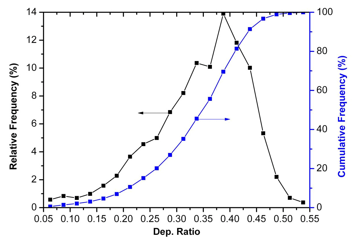
For ice phase clouds, DR is a good criterion for cloud boundary detection. The LIDAR measurements demonstrated that the peak value of DR in cirrus clouds in spring over Hefei varied from 0.2 to 0.5[3]. The DR shown in the bottom panel in Figure 2 can be used to validate the cloud layers shown in the middle panel, which was obtained using the algorithm introduced in the section 2.1 of this paper. The relative and cumulative frequencies of
From figure 3, it can be seen that the algorithm introduced here can be used to detect the cloud boundaries well. The algorithm seems to be reasonable and practicable, but it is impossible for ground-base Mie LIDAR to detect all kinds of clouds exactly because of limited information provided by only one tool.
3.2. Signal modification and inversion
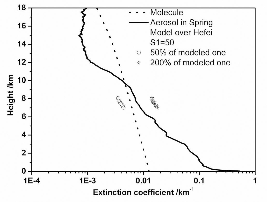
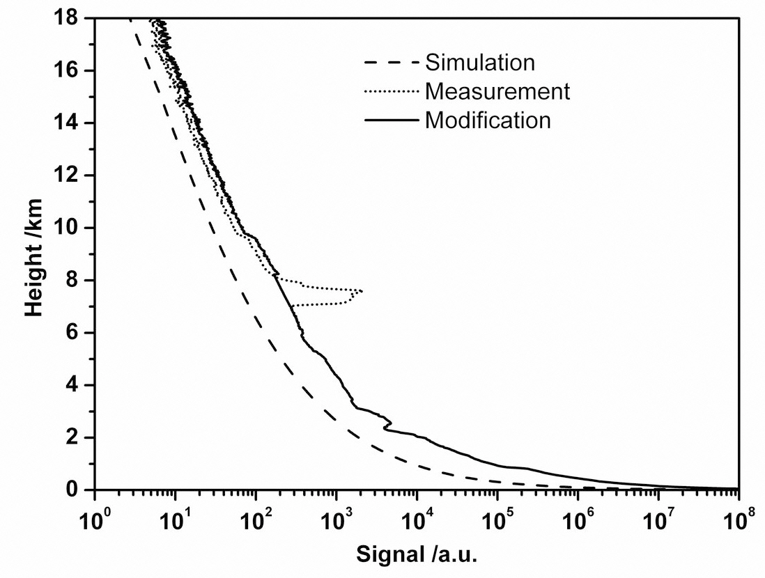
As presented in the algorithm part, suitable aerosol and molecular model data should be used to get a simulated signal. Figure 4 gives the modeled aerosol and molecular extinction coefficient data from the ground to 18km. And
the 50% (circle line) and 200% (star line) bias of the model,which are used in the next part as an error analysis in the detected cloud region are also shown in figure 4. Molecular data is derived from U. S. Standard Atmospheric Model and Rayleigh scattering theory. Aerosol data is derived from the routine measurement of troposphere aerosol in cloudless and fair nights during 1998-2008 by a 532 nm Mie LIDAR over Hefei. In figure 4, only spring data are used for this statistical aerosol extinction profile. Adding the LIDAR system parameters, a simulated signal, which shown in figure 5,(the dashed one) is created from Mie LIDAR equation,. In figure 5, the dotted profile is a observed signal by PML over Hefei at 18:49 LST on Mar. 9th, 2009 and the solid one is modified one using simulated signal, model data and detected cloud layer information. It is obvious that the signal after modification contains only aerosol and atmosphere information and the influence by cloud in inversion can be eliminated.
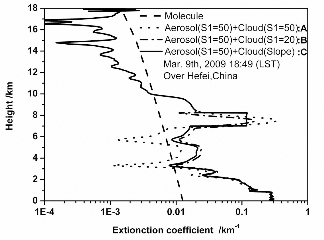
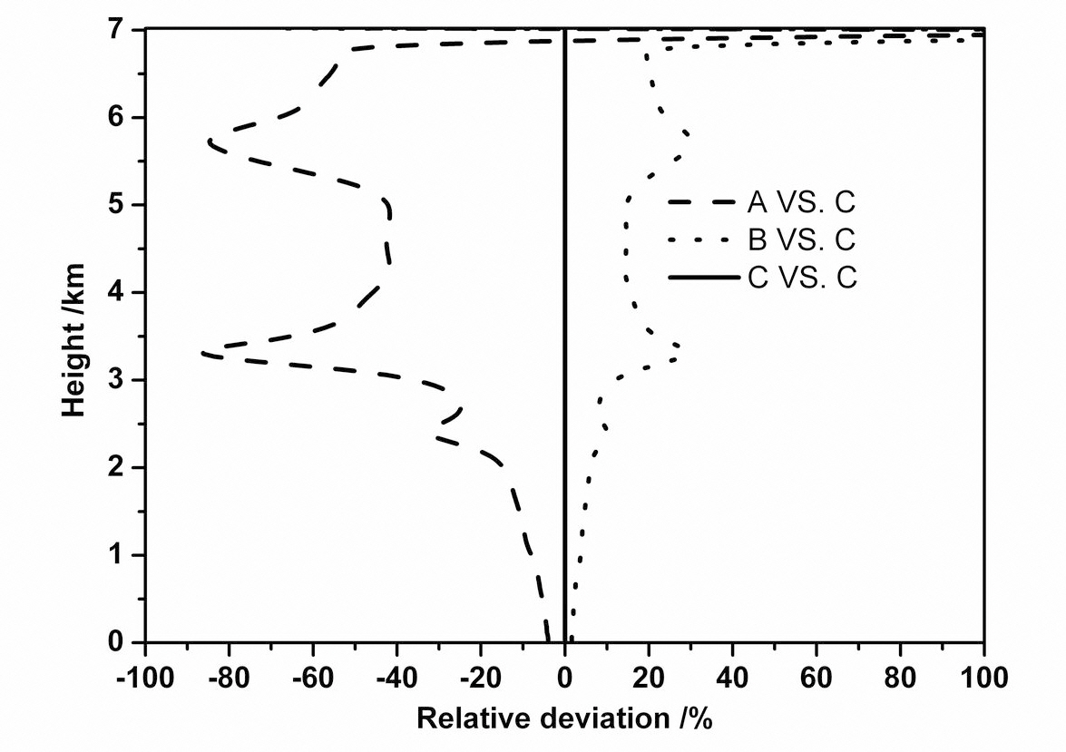
In order to compare this method with the traditional method, the measured signal and the modified one are inverted using the Fernald method. The aerosol extinction coefficient profiles from 0 to 18 km are derived from the
two kinds of signals: the dotted one (marked A) in figure 6 is directly derived from measured signal assuming
Figure 7 gives the relative deviation of profiles A and B compared with profile C below the cloud layer. The influence of the cloud layer on aerosol extinction is obvious and it makes the inverted results big or small by assuming a different LIDAR ratio. Sometimes, this relative error is more than 80%, especially in thin aerosol layers. So, the aerosol extinction by our algorithm is better than the one by the traditional method though it is improved (e.g. B is better than A in figure 7) through adjusting the LIDAR ratio of the cloud region.
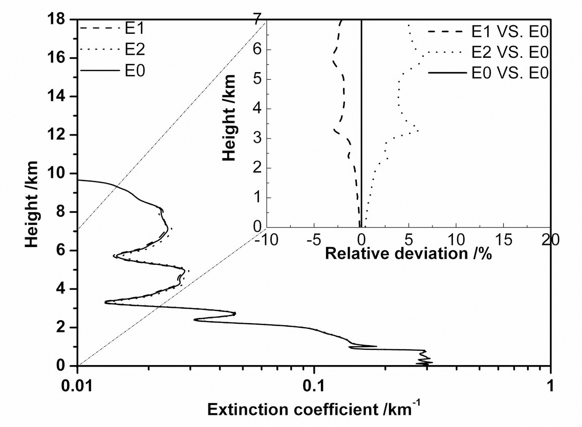
In our algorithm, a statistical or modeled profile is substituted in by matching conditions above and below the cloud layer. However, the actual aerosol conditions for these two locations can vary considerably between the statistical or modeled one, either thinner or denser. In this section,some analysis about the effect of this assumption made in the algorithm will be presented. As we know, the modeled aerosol extinction profile is needed for the simulated signal and then used for the modified signal. In order to emphasize what distortions in the retrieved result will be caused, the 50% and 200% bias of the modeled aerosol extinction in the cloud region (shown in figure 4) are used to create another two simulated signals. By using our algorithm and the Fernald method, three different inverted profiles as
shown in figure 8 are derived from the three modified signals. Here, the dashed line (marked E1), the dotted one(marked E2) and the solid line (marked E0) are related to 50%, 200% of the model and the model itself, respectively,as mentioned in the above paragraph. There are only a few differences among these three extinction coefficient profiles in the cloud layer region and below it. In the top right corner of figure 8, the relative deviations of profile E1 and E2 compared with profile E0 below the cloud layer are also given. The effects of assumed aerosol data in the cloud region on the inverted profile are not obvious.And the distortions of the inverted profile by increase or decrease of modeled aerosol extinction in the cloud region are less than 10%. The maximum of this relative error is only about 6.6% in a thin aerosol layer. So, the aerosol extinction derived by our algorithm is proved to be better than the traditional method and the relative error due to aerosol model substituting is acceptable.
The problem of the analysis of Mie-LIDAR signals from aerosol under a cirrus cloud has been addressed. Cloud and aerosol have different LIDAR ratios. The traditional Fernald method can not be used directly to retrieve accurate aerosol extinction from the LIDAR signal assuming a constant LIDAR ratio. Accurate determination of aerosol extinction under a cirrus cloud requires that the cloud boundary be considered, and that the value of LIDAR ratio for the cloud be also known. But the LIDAR ratio for the cloud can not be determined accurately. So, an improved algorithm to determine aerosol extinction below the cirrus cloud from Mie-LIDAR signals is developed including a cloud boundary detection method, a signal modification method, and the traditional Fernald method.
A method for detecting cloud boundaries has been presented, where some thresholds are used to find possible layers and to distinguish cloud layers from aerosol layers based on much quicker temporal variations of signal from cloud. The method is applied to the LIDAR data measured by PML, and the detected cloud features are validated by depolarization properties of the cloud. The algorithm for modifying LIDAR signals has been described in detail. The measured signal from the cirrus cloud is replaced by a simulated signal and the measured signal above the cirrus cloud is corrected using the transmittances of the simulated atmosphere layer and the detected cloud layer. Then the aerosol extinction under the cirrus cloud is derived from the modified signal and is tested and found to be better than the traditional method. The error due to aerosol model substituting is less than 10% in our present example.
The algorithm discussed in this paper is very useful in analyzing lots of real-time Mie-LIDAR signals automatically and continuously, and the information about aerosol and cloud can be found separately for further study.