In this paper the object recognition performance of a photon counting integral imaging system is quantitatively compared with that of a conventional gray scale imaging system. For 3D imaging of objects with a small number of photons, the elemental image set of a 3D scene is obtained using the integral imaging set up. We assume that the elemental image detection follows a Poisson distribution. Computational geometrical ray back propagation algorithm and parametric maximum likelihood estimator are applied to the photon counting elemental image set in order to reconstruct the original 3D scene. To evaluate the photon counting object recognition performance, the normalized correlation peaks between the reconstructed 3D scenes are calculated for the varied and fixed total number of photons in the reconstructed sectional image changing the total number of image channels in the integral imaging system. It is quantitatively illustrated that the recognition performance of the photon counting integral imaging system can be similar to that of a conventional gray scale imaging system as the number of image viewing channels in the photon counting integral imaging (PCII) system is increased up to the threshold point. Also, we present experiments to find the threshold point on the total number of image channels in the PCII system which can guarantee a comparable recognition performance with a gray scale imaging system. To the best of our knowledge,this is the first report on comparisons of object recognition performance with 3D photon counting & gray scale images.
Three-dimensional (3D) integral imaging and its applications have been investigated for 3D sensing, visualization, display,and recognition of objects [1-12]. This technique records 2D elemental (or multi view) images of a 3D scene for 3D image reconstruction and depth extraction. Both optical and numerical reconstructions are possible [10-11, 13]. Recently,photon counting integral imaging has been explored for 3D object reconstruction and recognition for photon-starved scenes. A variety of techniques, including maximum likelihood estimator and statistical sampling theory were applied for 3D imaging and recognition of photon-starved objects, respectively,using a fixed number of elemental images [13-15].
In this paper, we quantitatively compare the object recognition performance of a photon counting integral imaging (PCII)system with that of a conventional gray scale imaging system.Elemental image detection is based on a conventional photon counting model generating different Poisson numbers for each elemental image. A computational ray back propagation algorithm and a parametric maximum likelihood estimator[16] are applied to the photon limited elemental images in order to reconstruct the 3D scene. The performance of photon counting image recognition is evaluated by measuring the correlation peaks between the reconstructed 3D scenes.The photon-limited 3D reference object is computationally reconstructed to synthesize a matched filter. Normalized correlation peak values are calculated for the varied and fixed total number of photons in the reconstructed sectional image in order to compare the photon counting recognition performance obtained by changing the total number of the image channels in the PCII system. These results are compared with conventional 2D image recognition using gray scale images. We quantitatively illustrate that the object recognition performance of PCII system can be similar to one obtained by using a general gray scale image as the number of the image viewing channels in integral imaging system is increased up to the threshold point. Also, we show that the threshold point on the total number of image channels in the PCII system, which guarantees a comparable recognition performance with gray scale imaging system, can be found using a statistical sampling distribution of the measured average correlation peak values.
II. OBJECT RECOGNITION WITH PCII SYSTEM
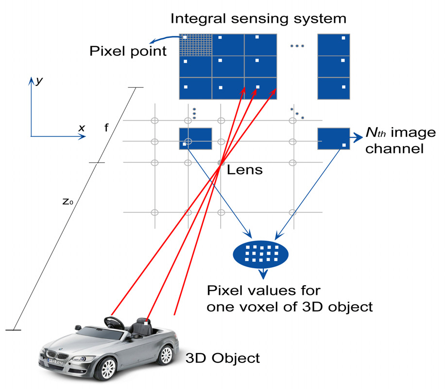
Fig. 1 shows a schematic setup of the integral sensing system with multiple image channels. The scene with very low intensity level light generates the photon counting elemental images. For 3D sensing of photon limited object,the system may utilize a single sensor with lenslet array, a sensor array, or a single moving camera in order to record the low intensity level light ray emanating from a 3D object. Each sensor captures its own photon counting two-dimensional(2D) elemental (perspective) image, which contains directional
information of the 3D object. The irradiance of one voxel on the surface of the photon limited 3D object is recorded on the corresponding pixel position of each photon limited 2D elemental image. Numerical 3D reconstruction of the original object can be performed by applying computational ray back propagation algorithm and parametric maximum likelihood estimator (MLE) to the recorded photon counted elemental images [13]. The pixel values on each elemental image corresponding to one voxel of the photon limited 3D object are assumed to be a random variable following a Poisson distribution function [17]. It is previously shown that one voxel value of the original 3D object can be retrieved by applying the parametric MLE to the elemental images pixel values as follows [13]:
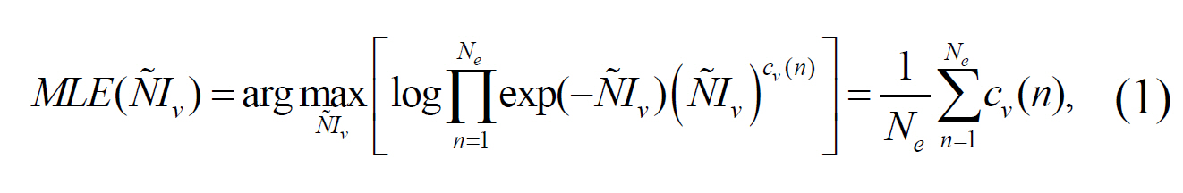
where
In order to evaluate the object recognition performance of PCII system, a matched spatial filter is applied to the sectional images reconstructed by using the integral imaging technique as follows [18]:
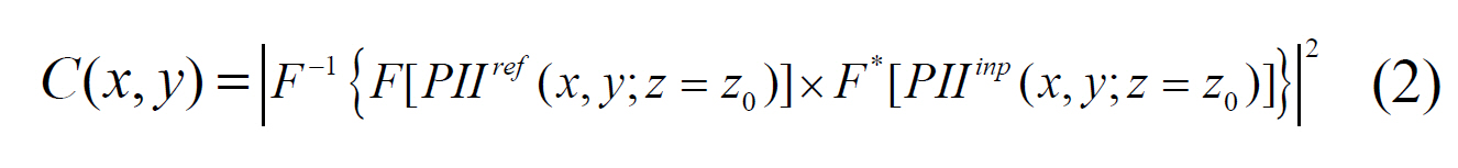
where
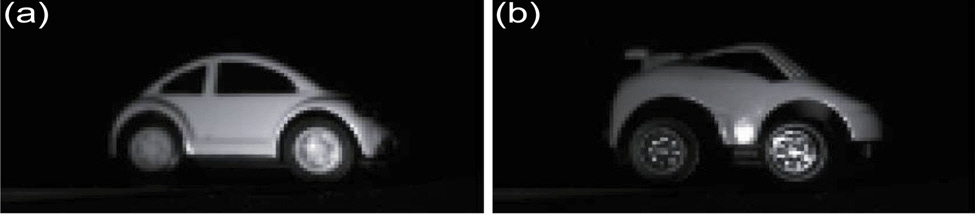
Experiments to evaluate and compare object recognition performance of an imaging system based on a conven tional photon counting model are presented. We recorded 9×9 elemental images for two toy cars by moving a CCD camera transversally in both x and y directions as shown in Fig. 1. Two objects denoted as car I and car II are used as two different classes of data for recognition (see Fig. 2).
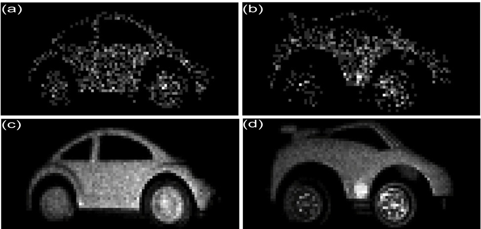
According to the classical photon counting detection model, the photon-counting elemental images of the toy cars were generated from the recorded elemental images,respectively [13]. Then, the sectional images of the 3D scenes for toy cars I and car II were reconstructed at a distance of z0 = 100cm with their corresponding photoncounting elemental images. We vary the expected number of photons in each input scene to test the recognition performance of the PCII system. Figure 3 shows the sectional images reconstructed from the photon-counting elemental images of car I and car II, respectively.
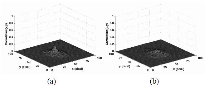
The matched filter in Eq. (2) was applied to the reconstructed sectional images in order to inspect object recognition performance of PCII system. Figure 4(a) shows the correlation plots of the photon counting image of car I in Fig. 3(a) used as a reference with the true class photon counting image as an input data. The true class input data was generated with the same expected number of photons (□=1000) and total number of the elemental images (
input data. For comparison, both plots are normalized to the same value that is the autocorrelation of the reference object. The measured correlation peak values were 0.21 and 0.12, respectively. It is noted that it is difficult to make a discrimination between car I and II by using only a single photon counting elemental image with the expected number of photons □=1000.
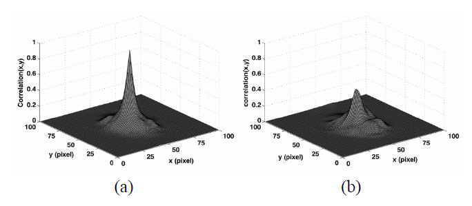
Figure 5(a) shows the correlation plots of the photon counting image of the car I in Fig. 3(c) as a true reference object (true class) with the true class photon counting image as an input data. The true class input data was generated with the same expected number of photons (□=1000) and total number of the elemental images (
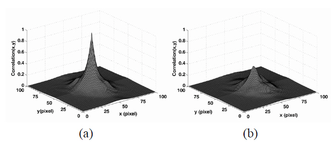
photon counting image of car I in Fig. 3(c) as a reference object with that in Fig. 3(d) for car II as a false class input data. Both plots (Fig. 5(a) and 5(b)) were normalized to the same value that is the autocorrelation of the true reference object. The measured correlation peak values were 0.97 and 0.46, respectively. For comparison, we present the auto-correlation and cross-correlation plots in Fig. 6 with the gray scaled intensity images of car I and car II in Fig. 2(a) and 2(b), respectively. The gray scale images in Fig 2 have the same view point as the photon counting images in Fig 3. Both plots (Fig. 6(a) and 6(b)) were normalized to the same value that is the autocorrelation of the true reference object. The auto-correlation and cross-correlation peak values calculated by using the conventional gray scale intensity images were 1.00 and 0.41, respectively. It is noted that when the total number of the image channels in the integral sensing system was increased to 81, the correlation plots between reference (car I) and unknown input photon counted images (car I and car II) become very similar to those between reference and unknown input intensity images in Fig. 2.
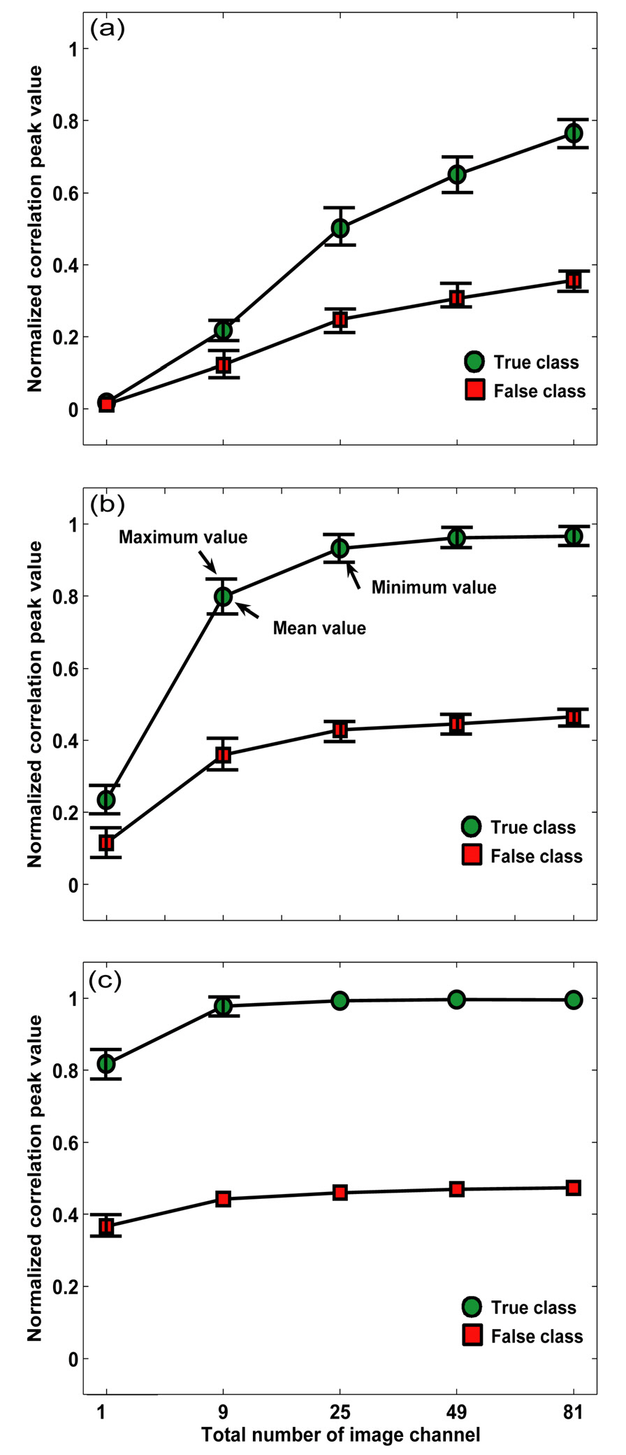
Figure 7 shows the correlation peak values computed between the photon counting sectional image of reference car I, and the photon counting sectional image of true class car I or false class car II. The correlation peak values were normalized to the same value that is the autocorrelation of the true reference object. The total number of elemental image
As shown in Fig. 7, the average correlation peak value between the photon counting sectional image of reference car I and the photon counting sectional image of true class car I approaches the auto-correlation peak value (=1.00) of the conventional intensity imaging in Fig. 2(a) when the total number of the image channel in the system was increased for fixed a number of photons. It is also noted that the average correlation peak value between the photon counting sectional image of reference car I and the photon counting sectional image of false class car II approaches the cross-correlation peak value (=0.41) calculated of the conventional intensity imaging of the car I and car II in Fig. 2(a) and 2(b) when the total number of the image channels was increased for fixed number of photons.These experimental results in Fig. 7 demonstrate that the increasing the number of the image viewing channels in PCII system can enable the recognition performance of PCII system to be similar to one of a conventional gray scale imaging system.
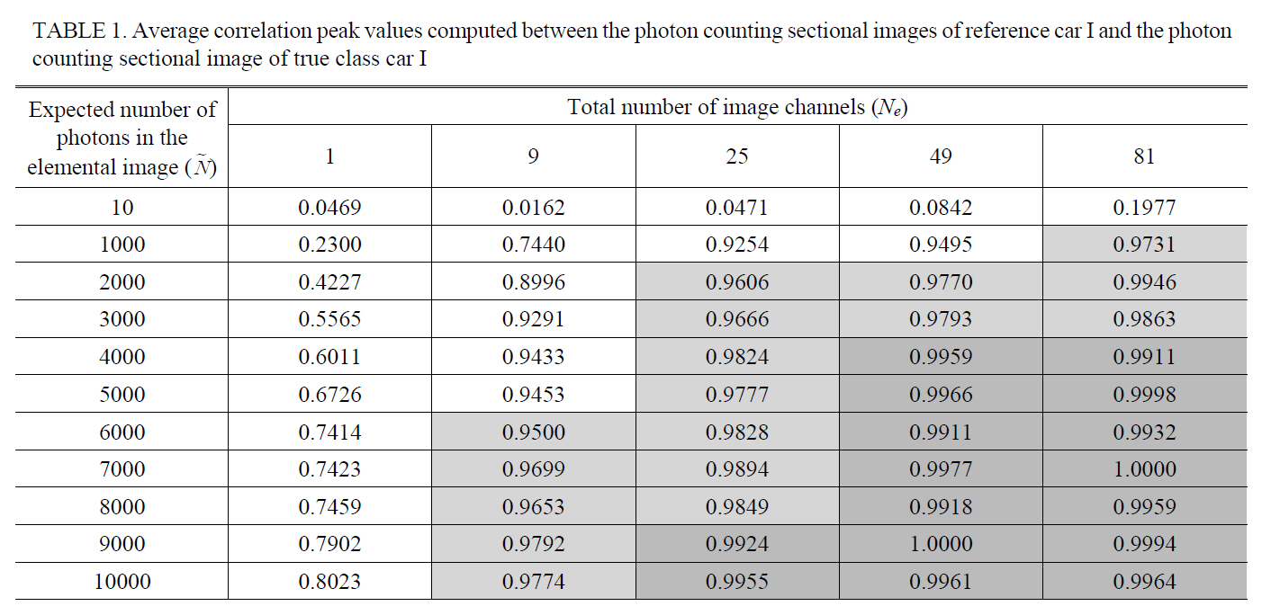
As the experiment to find the threshold point on the total number of image channels for the fixed averaged number of photons □ which guarantees a comparable recognition performance with gray scale imaging system,Table 1 and 2 show the average correlation peak values computed between the photon counting sectional image of reference car I and the photon counting sectional image of true class car I or false class car II changing the number of the image channels, respectively, where the expected number of photons in the photon limited elemental image was fixed as 10, 1000, 2000, 3000, 4000, 5000, 6000,7000, 8000, 9000, or 10000. The correlation peak values in the Table 1 and 2 were normalized to the same value that is the autocorrelation of the true reference object. The

Average correlation peak values computed between the photon counting sectional images of reference car I and the photoncounting sectional image of true class car I
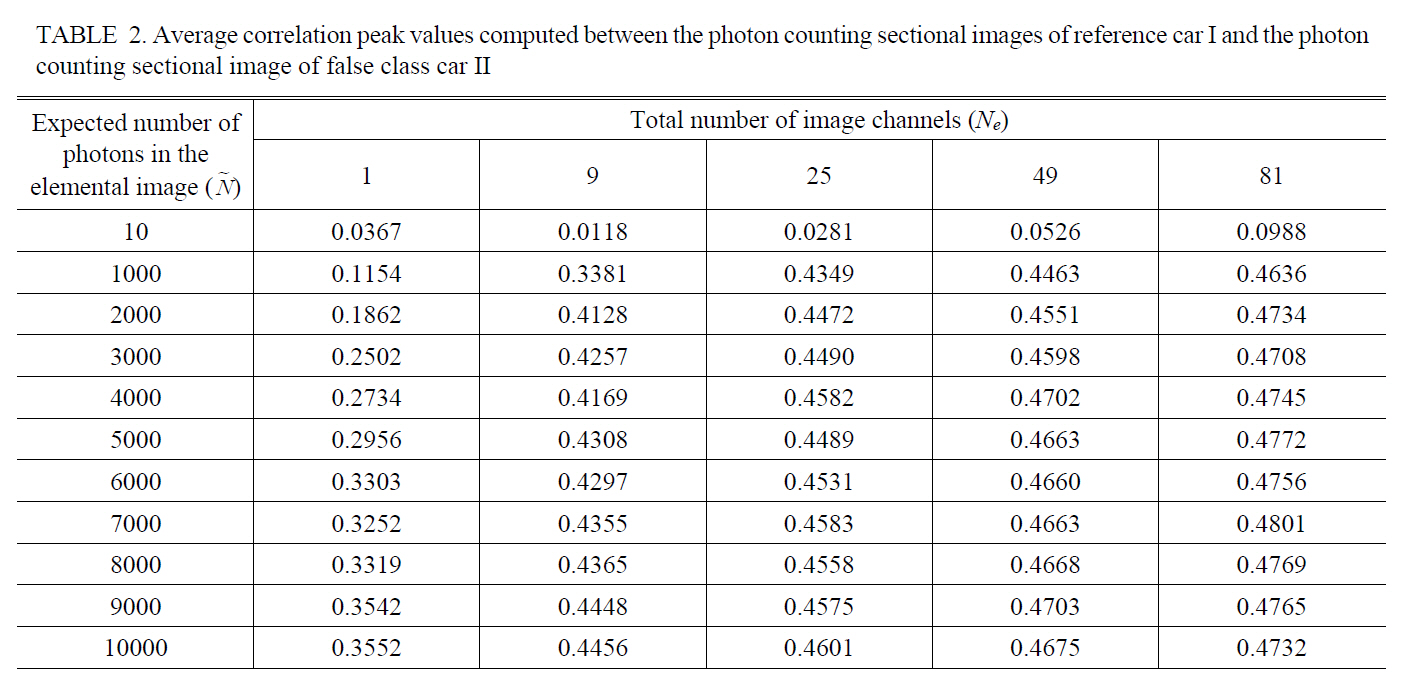
Average correlation peak values computed between the photon counting sectional images of reference car I and the photoncounting sectional image of false class car II
sectional image tested in the experiments has 125×125 pixels.It can be assumed that an arbitrary cut-off correlation value (for example 0.95 or 0.99) utilized in the conventional gray scale imaging system can be a possible decision criterion to evaluate the recognition performance in the 3D PCII system. Therefore, the threshold point on the total number of image channels for the arbitrary fixed averaged number of photons in the elemental image may be empirically found with the average correlation peak value measured in experiments. For example, if the average correlation peak value as the decision rule for an object recognition is set as 0.9500 or 0.9900 with the fixed averaged number of photons □=6000, the threshold point on the total number of image channels can be 9 and 49,respectively as shown in Table 1. It seems very difficult to derive the closed-form to describe the relationship between the optical parameters ( □,
The reconstructed sectional image can be characterized by the photon number per pixel, the total number of elemental images
In summary, we have quantitatively compared object recognition performance of PCII system with that of object recognition using conventional gray scale images. For visualization of a scene with small number of photons, integral imaging technique and parametric maximum likelihood estimator can be applied to the photon limited elemental image of the object. To evaluate photon counting object recognition performance, normalized correlation peak values between the reconstructed reference object and unknown input objects are computed for the varied total number of photons or the fixed one in the reconstructed sectional image changing the total number of image channels in the PCII system. The results are compared with those measured between the reference object and unknown input images obtained by conventional gray scale imaging system. It is shown that photon counting object recognition performance can be similar to one of conventional gray scale imaging system as the total number of the image channels in PCII system is increased up to the threshold point. Also, it is shown that the threshold point on the total number of image channels in the PCII system can be found using the statistical distribution of the average correlation peak values measured in the experiments. The PCII system to require less power consumption may replace the conventional imaging systems that generate gray scaled images for object recognition purposes.