Recently many research studies appeared on the moire effect in 3D displays, see, e.g. [1]. Among them in particular,various techniques were proposed to reduce moires: using filters [2], finding an optimal angle in the general (blackand-white) case [3] and especially for color displays [1].

For visual displays, the simulation of moires is also important because it provides an estimation of how much it can affect the spatial visual perception. For this purpose,finite observer distance and non-coplanar gratings should be considered. Other researchers have done simulations and related calculations for various displays including the following factors: the crossing angle and the relative velocity [4], the orientation of the brightness enhancement film [5], the finite gap between layers [1], and the shape by shadow moire [6] where the location of an observer is important.

In this paper we describe a polar representation form for moire waves based on their wavelength and orientation.Section II was presented at the conference [7] where we basically introduced the polar form for moires. In additional,we found analytical expressions for visible moires for the case of line gratings and an observer at a finite distance.Also, we described the computer simulation and the physical experiments, and we discussed a probable visual effect of moires on displayed 3D images.

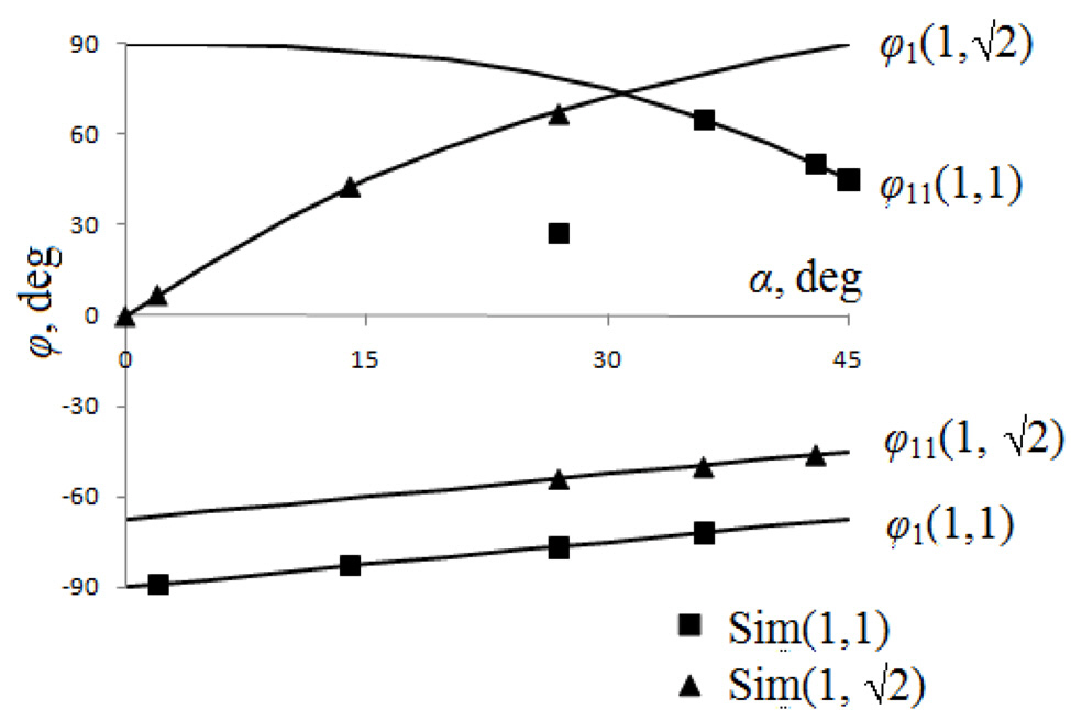
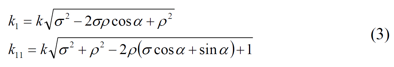
In the case of rectangular gratings, we have found [3]the two basic moire waves giving the strongest visual effect

where α is the angle between gratings, ρ is the ratio of the cell heights of two gratings, and σ is the aspect ratio of the rectangular cell.

The optimal angle (which corresponds to minimized wavenumbers)is the root of the quartic equation for s = sin α which includes σ as parameter. The exact solutions for three integer σ are α(1)=26.261°, α(2)=13.986°, α(3)=9.447°.

The orientations of the basic waves can be obtained from Eq. (1) as follows,

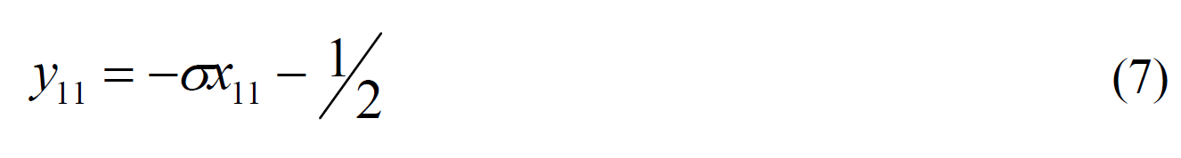
The wavenumbers of the basic waves have been found before [3]:

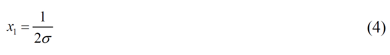
The wavelength can be obtained from Eq. (3) as a reciprocal value λ = 2π / k. Both wavelength and orientation can be drawn in a single graph using polar coordinates.For several values of α, the points may follow a curve. In the λφ-plane, the curves defined by Eqs. (2) and (3) turn out to be generalized circles (either straight lines or circles).

Under suitable conditions, one of the two generalized circles is a straight line, another is a circle. Namely, when ρ² = σ², the wave 1 is the line and the wave 11 the circle:

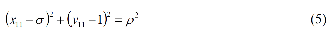
and when ρ² = σ² + 1, conversely, the wave 1 is the circle and the wave 11 the line:

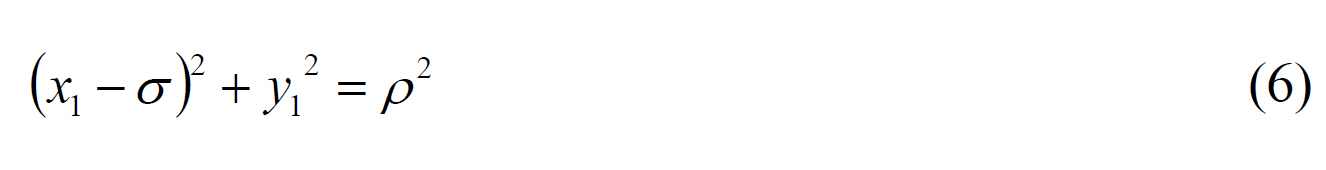
A distinctive feature of the curves (4) ? (7) is their spatial separation. When 0< α < π/4 (which is enough to consider with σ = 1), none of the above curves crosses the boundary between half-planes.

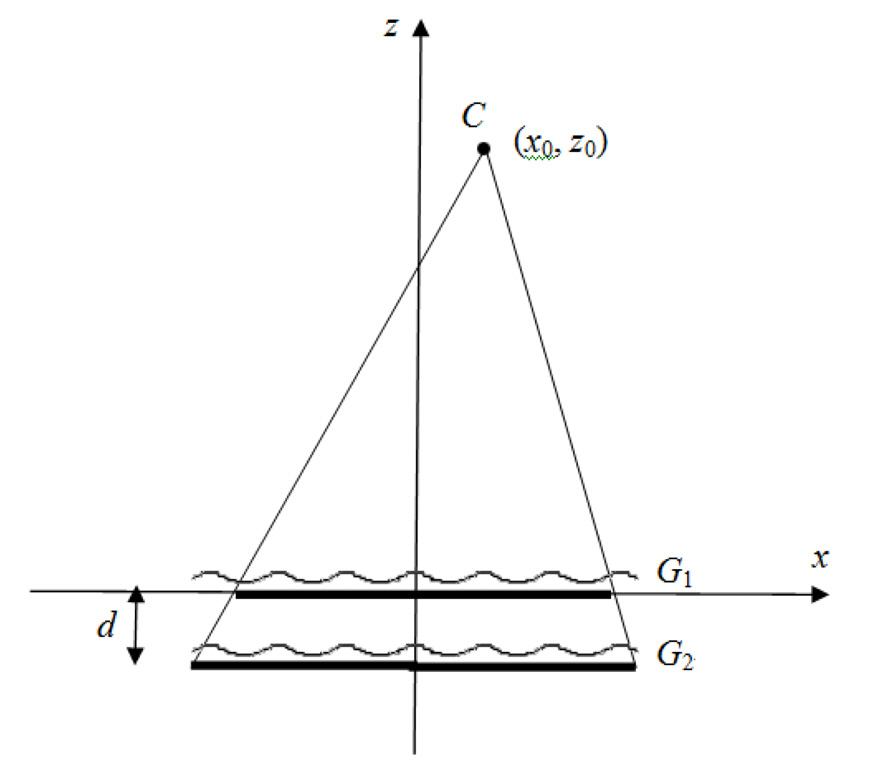
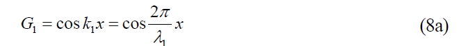
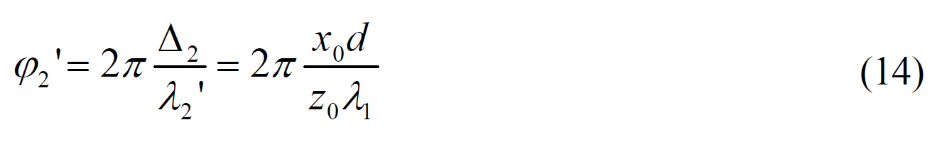
In this section we describe how the moire patterns appear for an observer located at a finite distance. Two parallel plain layers of regular structure (gratings) with a non-zero distance between them were simulated. The gratings with cosinusoidal transparence functions were used. In this paper we only consider wavelength and phase with no respect to the amplitude; thus we assume the unit amplitude. The following are the equations of gratings 1 and 2 (see also Fig. 1),

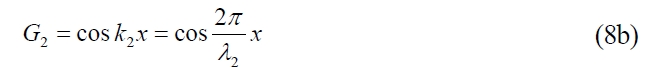
With a finite distance to an observer, one of the gratings can play a role of the screen, while another is effectively projected onto this screen through the projection center at C. The projection center is the location of an observer (or camera) which includes displacements x₀ and y₀. The following conditions provide an easier description of the projection transformation: the observer is at C = (x₀, y₀, z₀), the first grating in the xy-plane (z = 0), and the second grating in the parallel plane at -d. (It is also possible to locate the observer at the origin and express the data in the observer reference system by applying a translation transformation with more complicated formulas.) The geometry of projection is shown in Fig. 1. For this layout, the homogeneous transformation matrix looks like follows,

Using the matrix M, the transformation of the first grating G₁ (plane z = 0) is the identity transform, and this grating remains unchanged. The transformation of the second grating G₂ (plane z = -d) in Euclidean coordinates can be obtained by multiplication of the matrix (9) and the corresponding column vector. This yields,

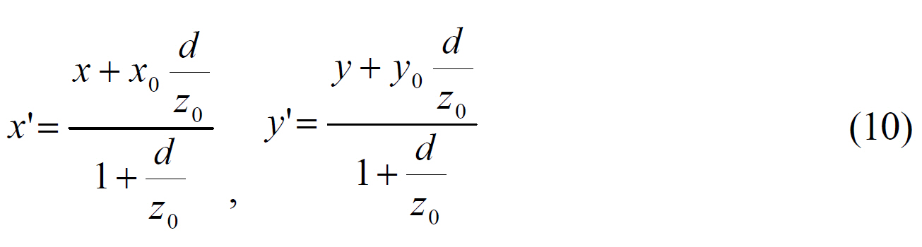
The Eq. (10) describes the transformation of coordinates only. Other meaningful physical quantities like a wavenumber,phase, etc. should be derived from it. In this paper we consider the line gratings and therefore y₀ = 0; also the wavelengths of the original gratings supposed to be equal: λ₁ = λ₂.

Since we assume the original gratings to be symmetric functions in respect to the x-coordinate as defined in Eq.(8), the result of transformation by Eq. (10) (without a lateral displacement) is also symmetric and can be represented by another cosinusoiudal function with a different wavelength. Then the ratio of coordinates equals the ratio of periods of symmetric functions. In other words, when the second grating is located farther from the observer than the first grating (as shown in Fig. 1), the transformed(projected) wavelength is reduced as follows,

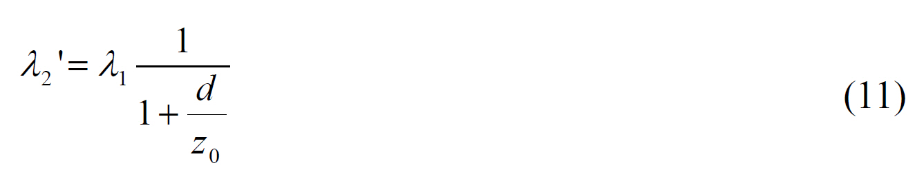
This yields the following expression for the transformed second grating with no lateral displacement:

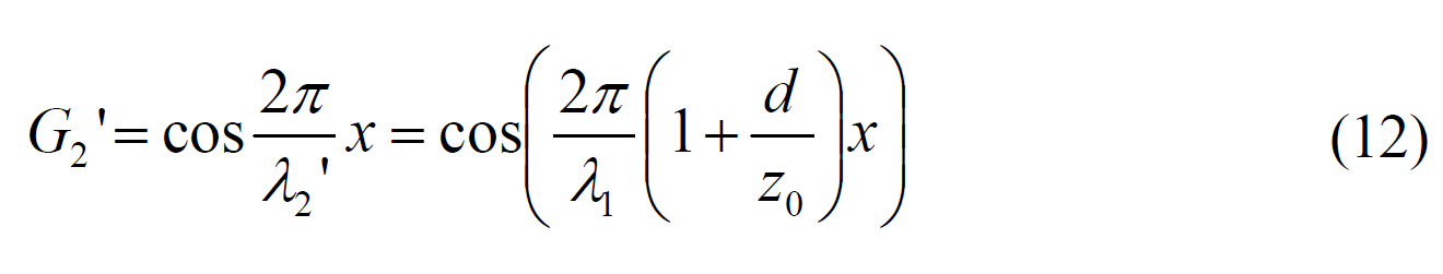
If an observer displacement is non-zero, x₀ ≠ 0, the expression for the displacement of the transformed second grating (with the wavelength by Eq. (11)) can be obtained from Eq. (10):

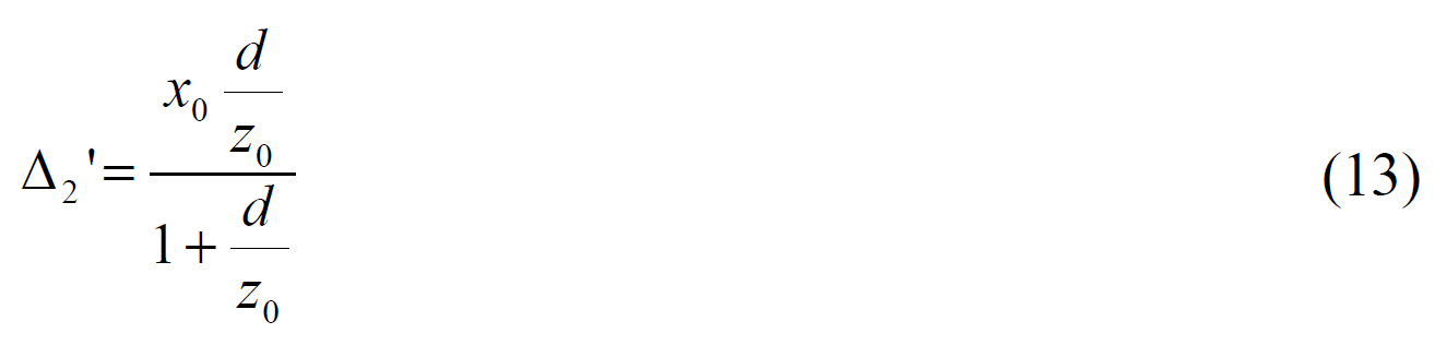
In this case, the projected second grating is non-symmetric,and there appears a phase difference between it and the symmetric grating obtained above, Eq. (12). The dimensionless phase difference can be expressed in terms of the dimensionless period 2π and thus can be found as the ratio of the displacement Eq. (13) to the wavelength Eq. (11)with a proper coefficient,

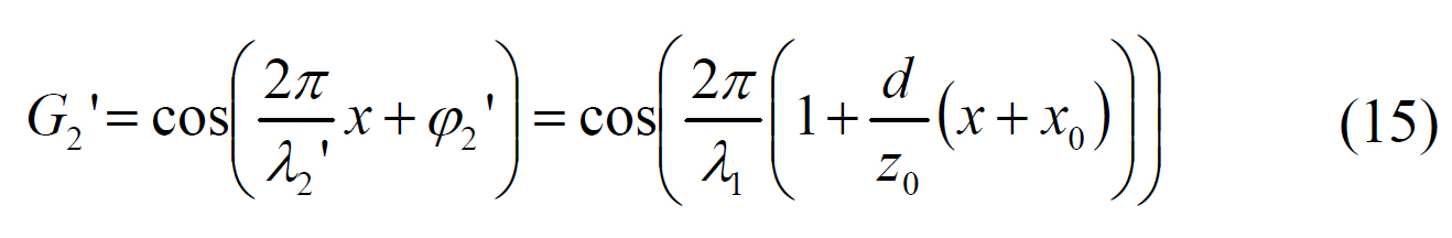
The resulting equation for the transformed second grating with a lateral displacement looks like the following:

Formulas (8a) and (15) effectively represent the gratings in the same plane, where they can be easily superimposed.The period and phase of the visible moires can be found by known formulas [8]. In our notation, the formula (2.11)from [8] looks like

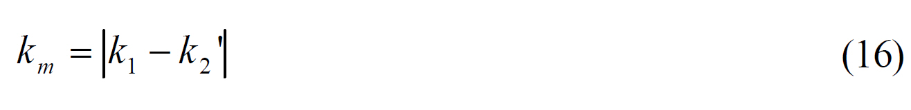
For the layout Fig. 1, the phase shift is zero, which means that the moire wave moves laterally in the same direction as the observer. From Eqs. (16) and (11), one can obtain the wavenumber

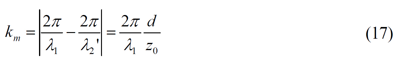
and the corresponding wavelength

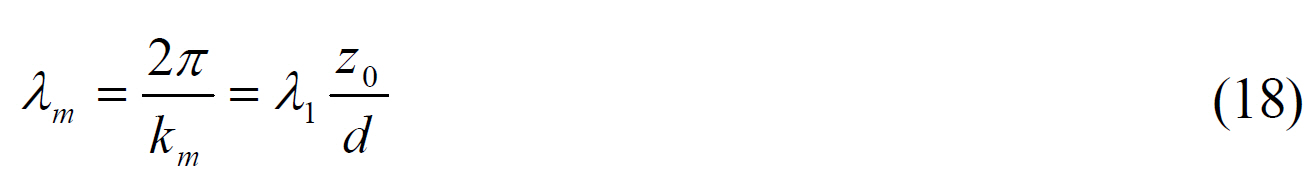
The formula (18) shows that the wavelength of visible moire is z₀/d times longer (because as a rule z₀ > d) than the original wavelength of the first grating. In particular, Eq. (18) gives an infinitely long moire wave for d = 0 which corresponds to the singular moire-free state [8].

The phase of the visible moire can be found from phases of the superimposed gratings by the formula (7.25) from[8], which indicates that when one grating is moved by a certain part of its period, the moire is moved by the equal part of the moire period. (N.B. The movement takes place along the corresponding wavevector.) This means that in the case of the parallel gratings of equal period at nonzero distance, the visible displacement of moire fringes is equal to the lateral displacement of the observer,

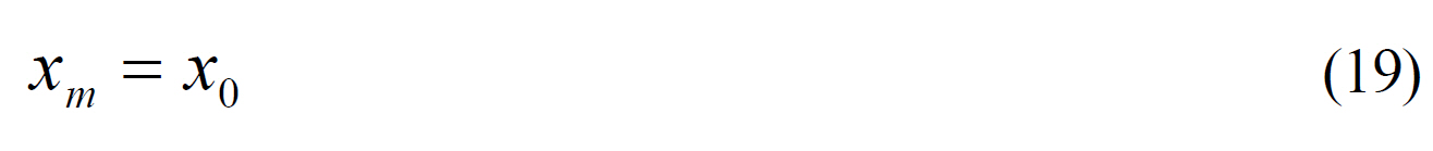
On the other hand, in respect to the lateral displacements,it can be said that this formula also describes the behavior of an image of an observer reflected in a plain mirror installed at z₀ /2, the halfway to the xy-plane.

When either of parallel line gratings is moved, the dimensionless phase of the visible moire is equal to the phase of the moved grating. Therefore the phase shift given by Eq. (14) can be included in the equation of the visible moire as follows:

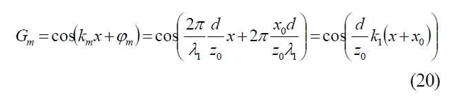
Eq. (20) shows that in the asymmetric case (when x₀ ≠0), the phase shift is proportional to the displacement x₀ with the same coefficient as the wavenumber. Also, the behavior of moires is different in respect to displacement x₀ and the distance z₀.

The preliminary simulation experiments were reported in[7]. In the current paper we present experiments of two kinds:the computer simulation and the physical experiments with real gratings when the gratings (ps-files for better accuracy)were installed between the covering glasses. The experimental setup is shown in Fig. 1. It includes the camera at C = (x₀, 0, z₀) and two gratings: G₁ at z₁ = 0 and G₂ at z₂ = -d (in this paper we only consider _y0 = 0). This is a modified layout from [9]. The upper grating (_G1 in Fig. 1)was printed on transparency. This grating could be either rotated along the z-axis or installed at fixed distances along it. The physical experiments were performed in two series: 1) d = 0 with the rotation angle α between 0 and 45°, 2) d ≠ 0 but α = 0. The first series represents the moires in the polar system while the second series relates to the finite-distance moires. In the physical experiments we used the sinusoidal gratings with periods 0.762 mm and 1 mm which were installed at d = 0, 2.75 mm or 4.25 mm.

The experimental data, the simulation for (σ, ρ) = (1, 1)and (1, √2) together with the corresponding theoretical curves Eqs. (4) - (7) are shown in Fig. 3 in polar coordinates.The wavelength in all graphs Fig. 3 is indicated in arbitrary units. It is convenient to assign the arbitrary unit to the shortest period of the gratings (0.762 mm in physical experiments and 6 pixels in simulation).

It important that experimentally (i.e. only based on the measured wavelength and the angle) it is virtually impossible to distinguish between waves 1 and 11. As mentioned above,the distinctive feature of the curves in Fig. 3 is their separation. In particular, none of them crosses the boundary between half-planes. The wave 1 (1, √2) and wave 11 (1, 1) lie completely in the upper half-plane; whereas the wave 1 (1, 1) and wave 11 (1, √2) lie in the lower half-plane.

The simulation of finite-distance moires was implemented by using the two-dimensional Fourier transformation. The images of two properly scaled and displaced line gratings(as it is described analytically by Eqs. (8a) and (15)) were superimposed (multiplied). After the Fourier transformation,the higher spectral components were excluded by using the concept of the visibility circle [8]. Then, the inverse transformation results in the visible moire. In simulation, the distance and displacement of the observer were considered as given values whereas the wavelength and displacement of moires were resulting ones.

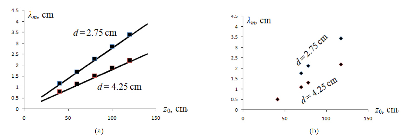
The results of this series of experiments are summarized in Figs. 4 and 5 as follows. The theoretical lines and simulations are shown in (a) while the results of the physical experiments with the real gratings are shown in (b). Fig. 4 shows the wavelength dependence on the observer distance.

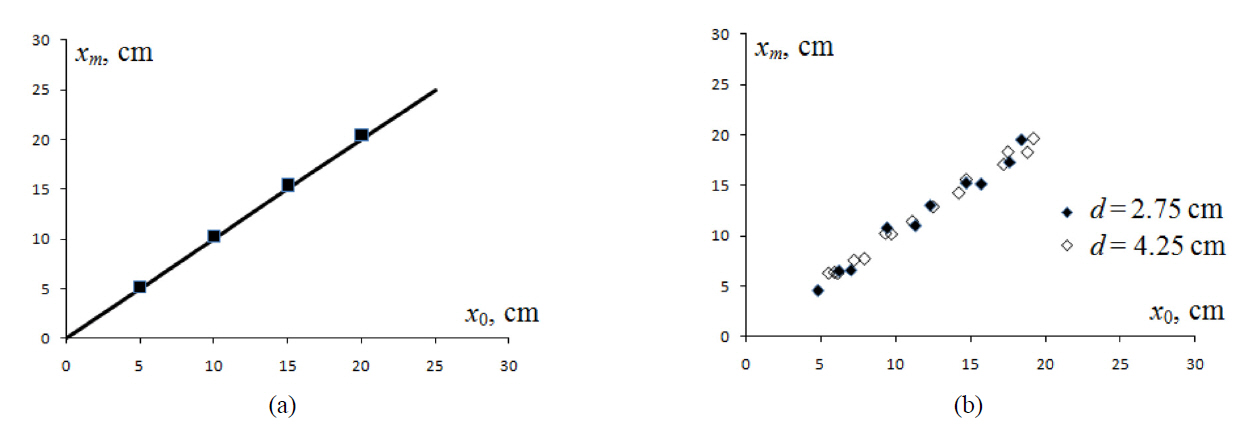
Fig. 5 shows the visible displacement of moires as a function of the lateral displacement of the observer. The data in Figs. 4, 5 are given for two values of the gap between the gratings, 2.75 mm and 4.25 mm. It seems to be important that none of graphs in Fig. 5 depends on d.

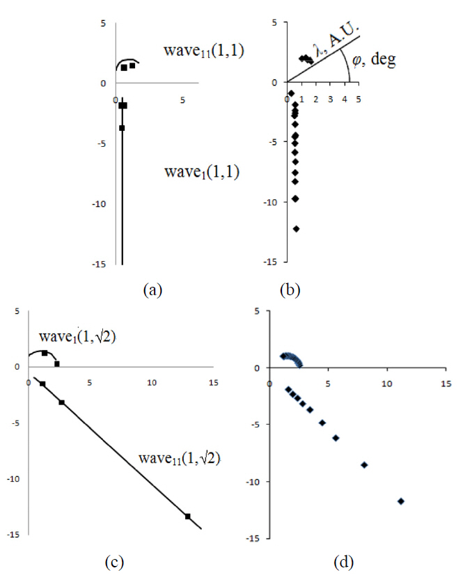
The suggested polar form seems to be convenient in describing moires by lines or circles in the λφ-plane.Conditions ρ² = σ² and ρ² = σ² + 1 (either generalized circle to be a straight line) are confirmed analytically. There is a good agreement (about 1°) between experimental and theoretical data excepting the close neighborhood of the minimization point where the difference exceeds 10° [7].This region may need additional investigation.

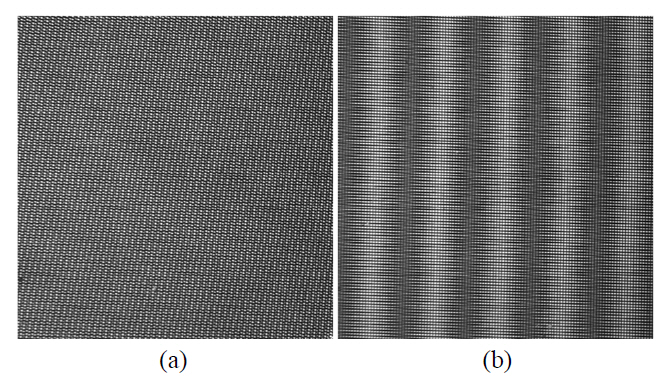
However the angles in the neighborhood of the optimal angle [3] were not included in the current results. The higher frequency and lower contrast ratio made recognition of moire waves in this limited region very difficult. Therefore the direct measurements of wavelength and angle of moires were not made for the rotation angle between approxi

mately 23° and 35°, see Fig. 6 where the photographs of moires obtained in experiments with overlapped gratings are shown within the neighborhood of the optimal angle and outside it. This corresponds to the loss of accuracy observed in [7] for this neighborhood.

When the observer, e.g., approaches the display, the moirewavelength becomes shorter by Eq. (18), and more moire bands appear within the screen. In practice z₀ ≫ d, so the change in the number of bands (say, from 20 to 21 bands per screen) may not be noticeable. On the other hand,when the lateral displacement x₀ is changed, the visible motion of moires is completely different; in particular,their wavelength remains unchanged. The lateral displacement of an observer by λ_m leads to the displacement of the moire by its period, as follows from Eqs. (18) - (20).This becomes especially clear for the moires with the period about several centimeters. When an observer moves laterally, the moire wave moves in the same direction and follows the smallest observer’s movement. This can make the change in moire appearance more evident than in the case of the changed distance.

The visible movement of moires does not follow a pattern for other objects normally displayed in a 3D display.Based on its motion parallax, the moire probably can be treated as lying in some plain behind the screen (though no other depth cue would confirm this). The visual behavior of moires for an observer approaching the screen may also be confusing, because the decreased wavelength can be sometimes treated as a more distant location. In this situation,the moire may seem to move away from the plane located by the motion parallax. Such ambiguous visual behavior might affect the other displayed objects and probably even disturb the stereoscopic perception.

The formulas for the period and phase of the visible moireare obtained for the case of two parallel line gratings. Both observer distance and the distance between plane gratings are finite and non-zero. The experimental graphs Figs. 4b,5b can fit the straight lines passing through the origin. The results of computer simulation correspond to the expression(19) for the visible moire wave. There is a good agreement between all three descriptions presented in this article: the theory, the computer simulation, and the physical experiments;it is within 2% - 3% for the theory and the physical experiment and less than 1% for the computer simulation.