In this work, for the first time, the quality of restoration in wide-field microscopy images after deconvolution was analyzed as a function of different Point Spread Functions using one deconvolution method,on a specimen of known size and on a biological specimen. The empirical Point Spread Function determination can significantly depend on the numerical aperture, refractive index of the embedding medium, refractive index of the immersion oil and cover slip thickness. The influence of all of these factors is shown in the same article and using the same microscope. We have found that the best deconvolution results are obtained when the empirical PSF utilized is obtained under the same conditions as the specimen.We also demonstrated that it is very important to quantitatively check the process’ outcome using several quality indicators: Full-Width at Half-Maximum, Contrast-to-Noise Ratio, Signal-to-Noise Ratio and a Tenengrad-based function. We detected a significant improvement when using an indicator to measure the focus of the whole stack. Therefore, to qualitatively determinate the best deconvolved image between different conditions, one approach that we are pursuing is to use Tenengrad-based function indicators in images obtained using a wide-field microscope.
Since its introduction in 1983, three-dimensional (3D)deconvolution microscopy has been a powerful tool for visualizing complex biological structures. This technique enhances resolution and contrast by using prior knowledge of a 3D point spread function (PSF) -which is the image of a single point source object through the optical path of the microscope-, to estimate the underlying spatial pattern of the fluorescent dye that gave rise to a measured image.Practically, the blurring function PSF can either be calculated using a theoretical representation of the microscope’s image forming optics or measured experimentally using sub-diffractionsized fluorescent particles. Therefore, it is very important to consider how the image formation process works in the microscope system.
1.1. Image Formation in an Ideal Microscope
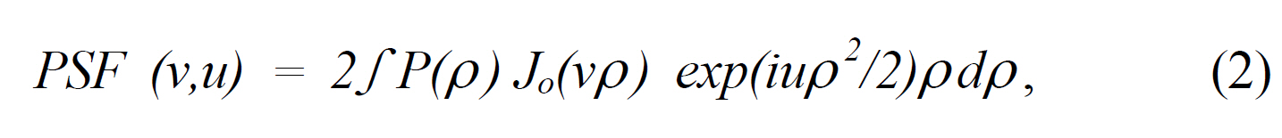
Theoretical models of the 3D imaging formation process in optical sectioning microscopy assume that the optical systems are free of aberrations [1]. In these ideal models,the PSF is linear and shift-invariant, which means that the image of a single point source is the same regardless of its position in the object space. Therefore, a single 3D PSF is sufficient to completely describe image formation throughout the 3D object space. An ideal aberration-free objective can be described in terms of the wavelike nature of light [2].A perfect lens transforms a spherical wave into another spherical wave. The image of the point source is a point image. The two-dimensional analytical formulation of the PSF of an aberration-free microscope [1] can be presented as follows:
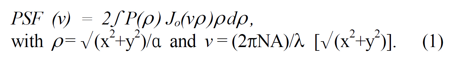
where P is the circular pupil function of radius a, J0 the first order Bessel function, λ the emission wavelength,NA the numerical aperture and x, y spatial coordinates.
Spherical waves interfere not only in the image plane,but also throughout the 3D space. Consequently, the image of the point source located in the object plane is a 3D diffraction pattern, centered on the conjugate image of the point source located in the image plane. With a perfect lens, this function is symmetric along the optical axis [3].The 3D analytical formulation of the PSF for a perfect,ideal, corrected and aberration-free objective is given by:
with u = (8π)/λ zη sin2 (α/2), η = refractive index, and α the half cone angle captured by the objective.
Along the optical axis, perpendicular planes present an intensity distribution similar in shape to the Airy disk.Similarly, axial resolution defines the minimum distance between two points in the z-axis. Unfortunately, this 3D image formation model has been shown to be inaccurate[4], especially for oil-immersion objectives of high NA.
1.2. Image Formation Using High NA Objectives
Shift invariance is not always demonstrated and PSF is all too often a function of the location of the point source in the object space. Most frequently, shift invariance does not apply in the axial direction. Axial shift variance results from the use of objectives under non-optimal conditions.This is unfortunately the case for the observation of thick biological specimens and particularly in living cell microscopy,in which the emitted light passes through media with different refraction indices [5].
Optical paths differ from the optimal path for which the objectives were designed, generating spherical aberrations that can severely affect the ideal image of a point source[6]. In general, only the plane position just below a cover slip of a given thickness and refractive index and separated from the objective by oil-immersion of a specific thickness and refraction index will produce an aberration-free image,as predicted by classical image formation theory. Any object placed elsewhere is subject to spherical aberrations [7].
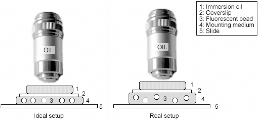
In practice, it is not easy to carry out microscopy in ideal conditions. For example (see Figure 1), the refractive index η of a living cell culture is closer to that of water(η=1.33) than to that of oil-immersion (η=1.516), and is far from the value for which optics are designed. Consequently,when light is focused deep into a cell well below the cover slip, it passes through various layers with different refractive indices, resulting in the generation of spherical aberrations.Spherical aberrations are characterized by axial asymmetry in the shape of the PSF, an increase in the flare of the PSF and a decrease in its maximum intensity [8]. Therefore, an
empirical PSF outweighs the theoretical PSF when using high NA objectives [5-8].
1.3. Deconvolution and the Empirical PSF
Deconvolution is a computerized inversion method for restoring an image distorted during the image formation process, based on prior knowledge of the degradation phenomenon. The deconvolution process is directly linked to image formation. The empirical determination of a PSF is a crucial step for the characterization of any optical system and a key preliminary step for image deconvolution. Therefore,the accuracy and quality of the PSF are essential to ensure the correct outcome of any deconvolution algorithm [9].
Previous experimental determinations of PSFs for fluorescence microscopy have revealed that empirical PSFs frequently exhibit strong radial and axial asymmetry [4], and thus differ significantly from the theoretical diffraction-limited PSF[2], [10-12]. Moreover, axial asymmetry has been proved to be due to spherical aberration that arises from an improper optical path length. Since microscope users are not always aware of the complexity of image formation and the influence of various factors on the imaging properties of their system,we will demonstrate in this article how the PSF is affected and how, in turn, deconvolution results are influenced.
We repeat and extend previous experimental studies about the empirical PSF determination showing that PSFs of high NA objectives (such as 40X and 100X) can significantly depend on the numerical aperture, refractive index of the embedding medium, refractive index of the immersion oil and cover slip thickness. The influence of all of these factors is shown in the same article and using the same microscope.For the first time, the quality of restoration after deconvolution was analyzed as a function of different PSFs using one deconvolution method, on a specimen of known size (a fluorescent bead) and a biological specimen (
This work mainly studies how the PSF quality affects the quality of images after deconvolution, using several imagequality indicators: Full-Width at Half-Maximum (FWHM),Contrast-to-Noise Ratio (CNR), Signal-to-Noise Ratio (SNR)and a Tenengrad-based function (TEN). Since deconvolution enhances high-frequency areas at the expense of low-frequency zones, assigns out-of-focus fluorescence to its correct spatial position and increases the degree of focus; deconvolved images will have better image quality indicators.
2.1. Microscopy System and Optical Sectioning
Raw images were obtained by optical sectioning using an Olympus BX50 upright microscope, equipped with a whitelight source for transmitted microscopy and a mercury UV-lamp for epi-fluorescence microscopy. Images were taken with a cooled monochromatic Apogee Instruments CCD camera Model AM4 of 14 bits of resolution, read noise of 10e, 768 pixel × 512 pixel sensor size, 9 ㎛ × 9 ㎛ pixel size, mounted to the microscope by a mount C lens(1X). This device has high-resolution and sensitivity, wide dynamic range, and good geometrical stability. A hybrid stepping motor (RS 440-436 1.8°/step) was connected to the micrometric screw of the microscope allowing a minimum movement of two steps (3.6º), resulting in a 500 nm theoretical resolution. A RS 718-896 reduction box(100 to 1) was attached to the motor to enhance resolution enough for optical-sectioning studies [13]. The CCD camera and stepping motor were controlled by specialized software(designed for the authors in Object Pascal language to control both the camera via an ISA card and the stepping motor via parallel port). The same software also included deconvolution algorithms and a 3D visualization interface[14]. Optical sectioning was automatically done after loading some basic parameters which included image dimensions,time of exposure, distance between in-focus planes and motor speed (which determined stage speed). The work was executed using corrected Plan-Apochromatic (UPlan Apo Universal-Olympus) either 40X dry (NA 0.85, determining voxels of 0.20 × 0.20 × 0.25 ㎛3) or 100X oil (NA 1.35, 0.10 ×0.10 × 0.15 ㎛3 voxel size) objective lenses. Then, the stage was moved upwards a distance equal to half the total depth of the future stack and the stepping motor was programmed to move it downwards in step of 0.25 or 0.15 ㎛ (for 40X and 100X, respectively). The time of exposition was the same for all samples.
Empirical PSFs were obtained using fluorescent beads(F-8888 kit; Molecular Probes, OR, USA). As a point source of light, we used fluorescent beads whose diameter must be less than the lens resolution (0.39 ㎛ and 0.25 ㎛ for 40X and 100X, respectively) [9]. Beads which were 0.11,0.18, and 0.46 ㎛ in diameter were selected (even though the last one, does not meet the criterion, it was selected to check the effect of bead size on PSF determination). The beads are coated by fluorophores with excitation/absorption peaks at 505/515 nm (same excitation peaks as for FICT(fluorescein isothiocyanate), the yellow/green fluorophore used in our experiments). Original solutions containing 0.11 ㎛,0.18 ㎛, and 0.46 ㎛ fluorescent beads were diluted in distilled water (1:100) so as to obtain disperse beads (and,therefore, images where a single one can be isolated and used as point source of light), and a 5 μL drop of each was placed on a cover slip and left aside until dehydration.Then, these cover slips were placed over slides containing a drop of mounting medium. When using the 100X lens, a drop of immersion oil (Olympus, America Inc., η=1.516)was placed on top of the cover slip. In order to obtain a good SNR, the camera was cooled down to -10℃, (to reduce electronic noise in the image acquisition process);and each image was an average of three captures at the same plane, which were then background corrected. For both objectives, a stack of 64 sections was sufficient to obtain the complete PSF. Each image was finally stored in TIFF format. The Full Width at Half Maximum (FWHM)parameter was used to determine resolution using these PSFs.
In order to assess PSF resolution under diverse optical paths,we obtained empirical PSFs under thirty different experimental conditions (five samples of each condition were selected for statistical purposes). Same acquisiton parameters (image

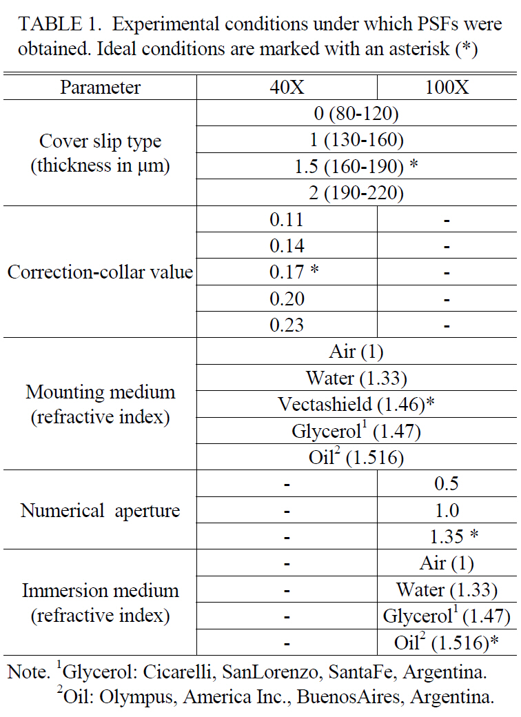
Experimental conditions under which PSFs wereobtained. Ideal conditions are marked with an asterisk (*)
dimensions, time of exposure, motor speed, number of averaged planes, number of sections, and background correction) were used for each condition. Thus, a whole range of different optical paths were studied ranging from nearly ideal through commonly used ones up to extreme cases (Figure 1). Table 1 summarizes the experimental conditions which were evaluated.
Images were deconvolved using a positive constrained iterative deconvolution method [3, 9]. It reassigns defocused information to its original position in the 3D image stack.Therefore, this method is useful when quantification is involved as in this case study. The general philosophy of iterative algorithms is to estimate a solution
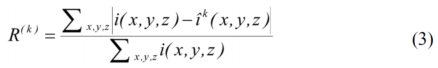
R(k) provides only a method for convergence.
The algebraic update method is based on the Van Cittert update scheme. The physical positivity restriction is also added to this scheme.
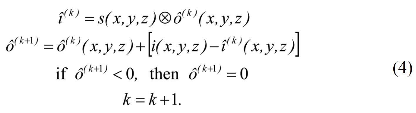
equation (4) shows the algorithm’s step by step sequence.The starting point is k = 0, where
2.4. Specimen Preparation and Sectioning
Two types of specimens were imaged: 4 ㎛ fluorescent microspheres (pattern specimen) and Rhinella arenarum whole embryos incubated with IgG-FITC-anti-E-cadherin(biological specimen).
The fluorescent microspheres (4 ㎛) were prepared according to the PSF-preparation protocol explained in the previous section using the ideal condition (see Table 1). Image stacks consisted of 32 or 64 optic sections (corresponding to 8 ㎛ and 9.6 ㎛ of thickness) of 128 pixel x 128 pixel 2D images for 40X and 100X objectives, respectively.
Stage-19 (Gosner, 1960 [16]) Rhinella arenarum embryos were treated to study the skin expression pattern of E-cadherin cell adhesion molecule, following Izaguirre’s protocol [17].They were fixed in Carnoy, washed in 1X PBS at room temperature (RT) and then treated with 0.1% Triton X-100(SIGMA Chemical Company, St. Louis, USA) in PBS during 30 minutes at RT. The samples were then incubated in goat normal serum 1:20 for 35 minutes followed by anti-E-cadherin antibody (mouse monoclonal antibody; Transduction Laboratories,Lexintong USA) 1:50 at 37℃ for 75 minutes. Next, embryos were washed in 1X PBS and incubated with the IgG-FITC(SIGMA) 1:64 at RT for 105 minutes, and then washed again with 1X PBS. Finally, they were mounted in Vectashield mounting medium (Vector Laboratories, Vector Burlingame,CA) to prevent the fluorophores decay. According to skin thickness (? 25 ㎛) previously determined in morphological studies [17], 128 (32 ㎛) and 256 (38.4 ㎛) optic sections of 256 pixel x 256 pixel were collected with 40X and 100X,respectively.
3D image quality was evaluated using four indicators:FWHM, CNR, SNR and TEN, in order to assess the quality of restoration after deconvolution [18-19]. FWHM was used to assess resolution (PSF) and z-axis elongation (pattern specimen) [13], while CNR, SNR, and TEN were used as general image quality indicators.
The FWHM parameter can be used to measure the diameter of spherical objects such as microspheres. Steps involved in the calculation of the FWHM are as follows. First, an intensity profile is obtained from a path traced through the object’s center point. Then, the maximum intensity value I is determined and the distance between the two points that correspond to an intensity equal to I/2 is provided as the FWHM; this value corresponds to the object’s diameter.The FWHM was measured along the X, Y and Z axes(dX, dY and dZ respectively).
CNR and SNR values are calculated using (5) and (6),respectively where the standard deviation of noise corresponds to those of all pixels with an intensity below a given threshold.
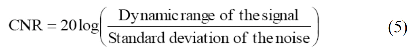
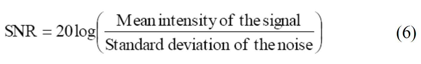
Where “Dynamic range of the signal” is the range that contains all values of meaningful fluorescence, “Mean intensity of the signal” is the average of all pixels with an intensity value withing the dynamic range and “Standard deviation of noise” is calculated by (6*):
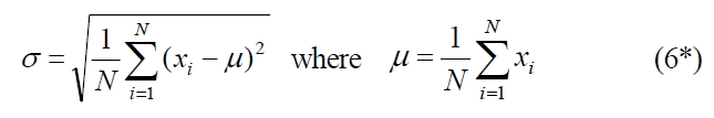
Where xi are the N noise values used to calculate the standard deviation σ. For the present work, we only consider background noise. The background noise range was established between the minimum intensity value (zero) and a maximum intensity threshold which was determined from out-of-focus images.
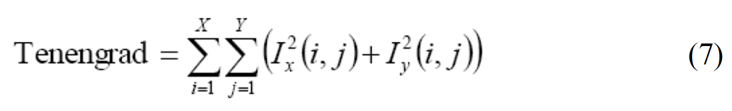
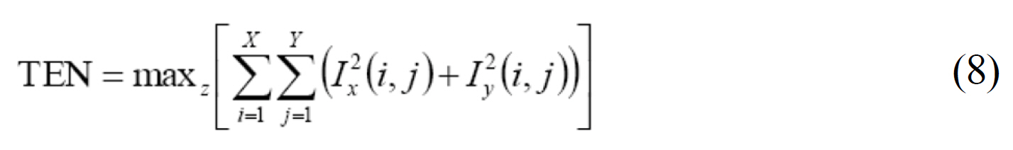
The Tenengrad function shown in (7) provides a value that indicates the degree of focus of a given 2D image,where Ix and Iy are gradient images which result from the convolution of the original image with the Sobel operators[20]. In order to work with 3D images, we propose the 3D Tenengrad-based indicator shown in (8).
The results are presented as mean ± S.D. In the statistical analysis, the FWHM and sphere diameter values, obtained using ideal and each non ideal condition were compared by t-test. The same test was utilized to compare CNR, SNR and TEN values. The level of significance employed was significant (*) p ≤ 0.05 and very significant (**) p ≤0.01. Data were analyzed with SPSS 10.0 software.
3.1. Microscopy System and Optical Sectioning
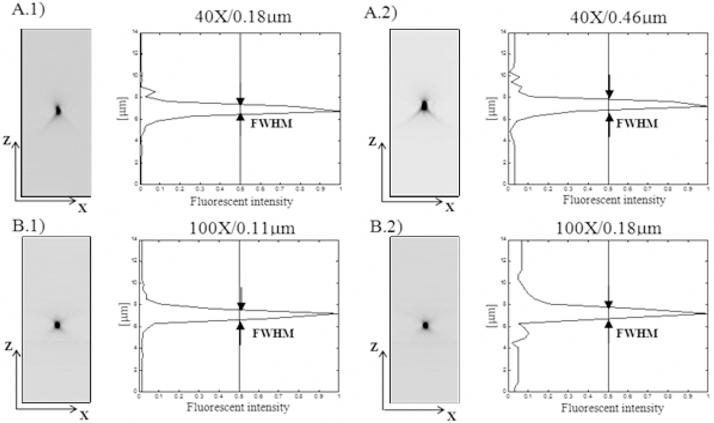
Figure 2 shows maximum projections of the PSF and its intensity profile along the optical axis for the ideal optical setup. With 0.18 ㎛ and 0.46 ㎛ fluorescent beads the measured FWHM were 1.54 ± 0.11 ㎛ and 1.85 ± 0.03 ㎛ respectively for 40X objective (Figure 2A), and with 0.11㎛ and 0.18 ㎛ fluorescent beads, the FWHM values were
1.10 ± 0.08 ㎛ and 1.12 ± 0.04 ㎛ respectively for 100X objective (Figure 2B). Each measurement represents an average over 5 different beads. These data show that the PSF appears slightly elongated along the Z axis but exhibits a considerably radial symmetry.
3.2. Empirical PSF Determination Under Different Conditions
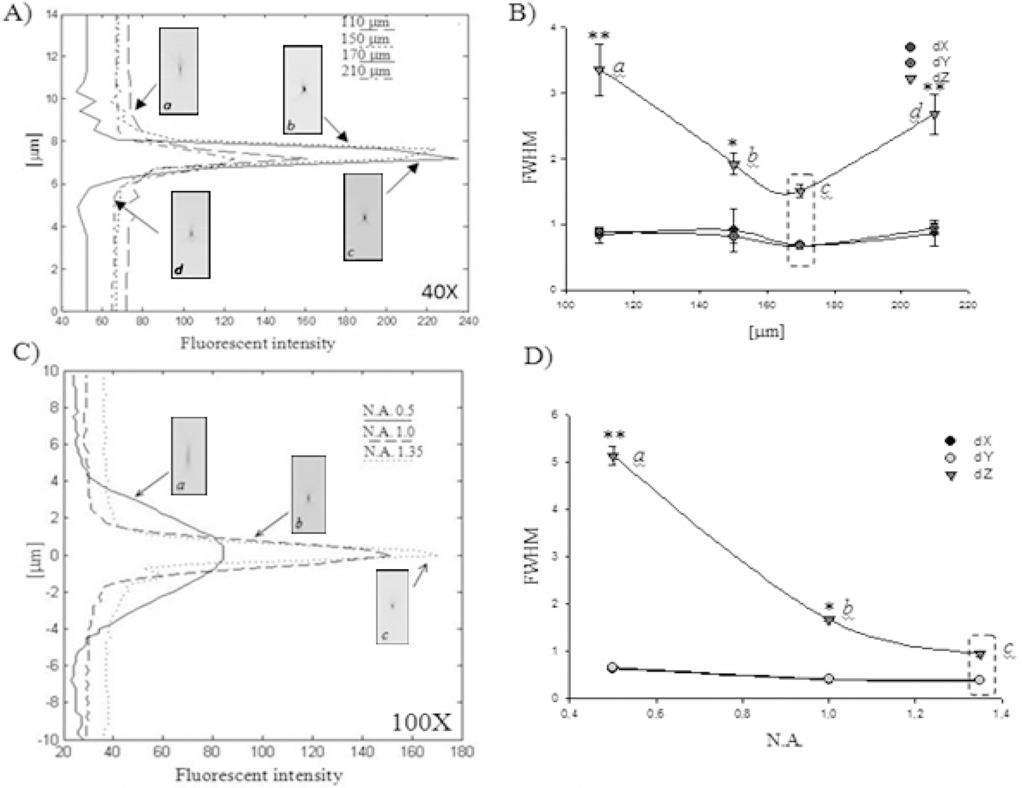
Figure 3 shows FWHM values as a function of cover slip thickness for the 40X objective and as function of numerical aperture for the 100X objective. Four different types of cover slip were used. Figure 3A shows the x-z cross-sections and the intensity plots of a 0.18 ㎛ microsphere.The PSF obtained using the optimal cover slip thickness(170 ㎛) (c) had the most symmetrical light distribution along the z-axis (resembling an “X” or an hour-glass).This cover slip also showed the least light dispersion (i.e.,most of the light was concentrated near the focal plane).PSFs obtained using other cover slip (a, b, and d) present an asymmetric distribution, resembling a “Y” shape. This experiment reveals two main effects of changes in cover slip thickness. Firstly, the peak intensity of the PSF decreased
when using a cover slip other than the one of 170 ㎛ of thickness, showing a maximum decrease when using the cover slip of 210 ㎛. Over a distance of 5 ㎛ we measure a decrease in the peak intensity of the PSF of more than 50%. Secondly, we observed a significant increase in the width of the PSF in the axial (dZ) but not the lateral (dX,dY) directions (Figure 3B). FWHM in the dZ direction was 1.51 ± 0.03 ㎛ (Figure 3B-c) for the optimal condition,and 3.36 ± 0.32 ㎛ (Figure 3B-a) (very significant), 1.92± 0.16 ㎛ (Figure 3B-b) (significant) and 2.68 ± 0.25 ㎛(Figure 3B-d) (very significant) for 110 ㎛, 150 ㎛, and 210 ㎛ thicknesses, respectively. Similar results were observed when we tested other conditions (correction-collar value and embedding medium). In general, we observed an increase in the width of the PSF in the axial direction when the conditions differed from the ideal one, while this did not occur in the lateral directions.
Using the 100X objective, three different values of NA were compared. Figure 3C shows x-z cross-sections and the intensity plots of a 0.18 ㎛ microsphere. The PSF obtained using the highest NA (NA=1.35) (c) had the most symmetrical light distribution along the z-axis. The peak intensity of the PSF decreased when NA diminished. Over a distance of 2 ㎛ we measured a decrease in the peak intensity of the PSF of more than 20% and 50% for NA=1.0 (b) and NA=0.5 (a) respectively. For the optimal NA, FWHM in the dZ direction was 0.95 ± 0.06 ㎛(Figure 3D-c) and 5.14 ± 0.20 ㎛ (Figure 3D-a) (very significant) and 1.67 ± 0.04 ㎛ (Figure 3D-b) (significant)for NA=1.35, NA=0.5, and NA=1.0, respectively. Other conditions for 100X objective also were tested using 0.11㎛ microspheres (numerical aperture, cover slip thickness,embedding medium and immersion medium) and using 0.18 ㎛ microspheres (cover slip thickness, embedding medium and immersion medium). Similarly to what was seen using the 40X objective, in all evaluated conditions we observed an increase in the width of the PSF in the axial direction when the conditions differed from ideal one, while the FWHM in the lateral direction did not vary.
3.3. Effects of Empirical PSFs on the Deconvolution of the Pattern Microsphere Images
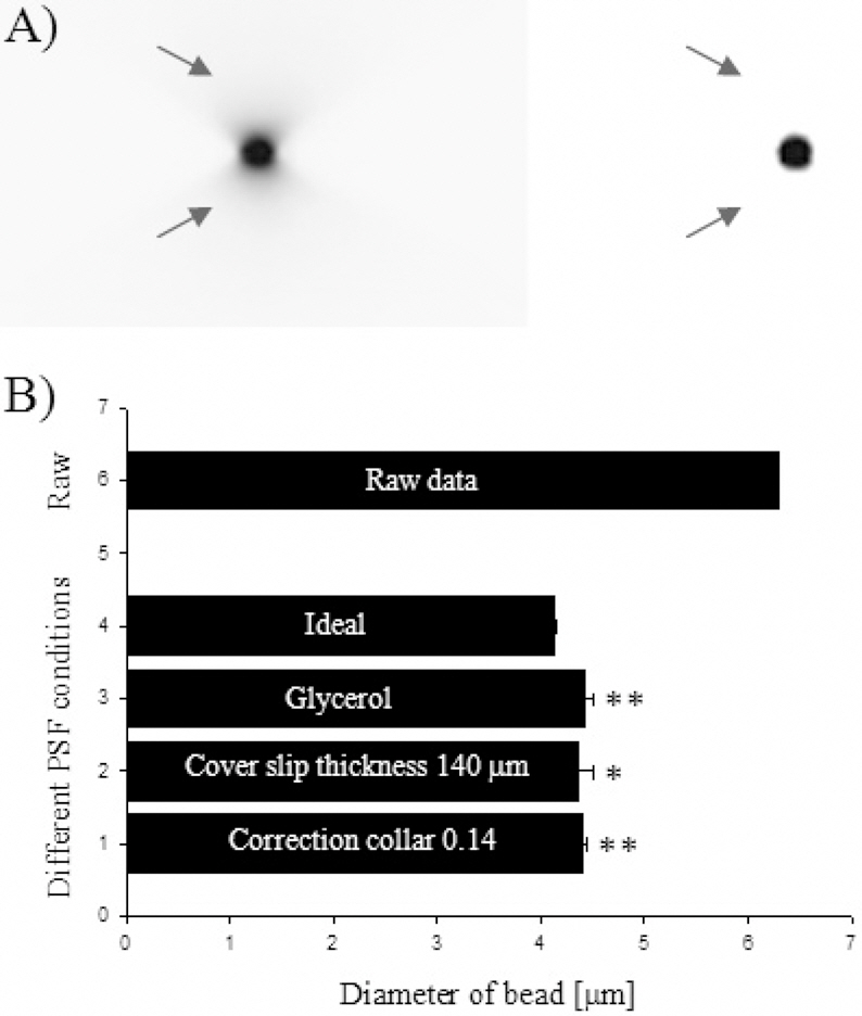
Using our system we took a 3D image of a 4 ㎛ fluorescent microsphere which was prepared using ideal conditions (40X lens, air, cover slip N° 1.5 (170 ㎛),Vectashield, microsphere, and slide). Figure 4A shows in the left panel an x-z projection of a raw 4 ㎛ fluorescent microsphere and in the right panel, their corresponding x-z projection of the same microsphere after deconvolution with an ideal PSF. The raw fluorescence image appears elongated axially (arrows) and after deconvolution this elongation is reduced nearly to the original diameter of the bead.Figure 4B shows a comparison between elongation reductions after deconvolution using the 40X objective. The raw data has a FWHM of 6.29 ± 0.01 while processed data’s value was reduced to 4.12 ± 0.03 ㎛ using an ideal PSF, 4.42± 0.06 ㎛ (glycerol, very significant), 4.36 ± 0.09 ㎛ (N°1(140 ㎛) cover slip, significant), and 4.40 ± 0.02 ㎛ (0.14 correction collar value, significant). Similar data were obtained working with the 100X objective (data not show).These results mean that for both objectives, the best results were obtained when deconvolution was performed using a PSF captured under ideal conditions.
3.4. Effects of Empirical PSFs on the Deconvolution of Rhinella Arenarum Embryo Images
The skin expression pattern of E-cadherin was studied in stage 19
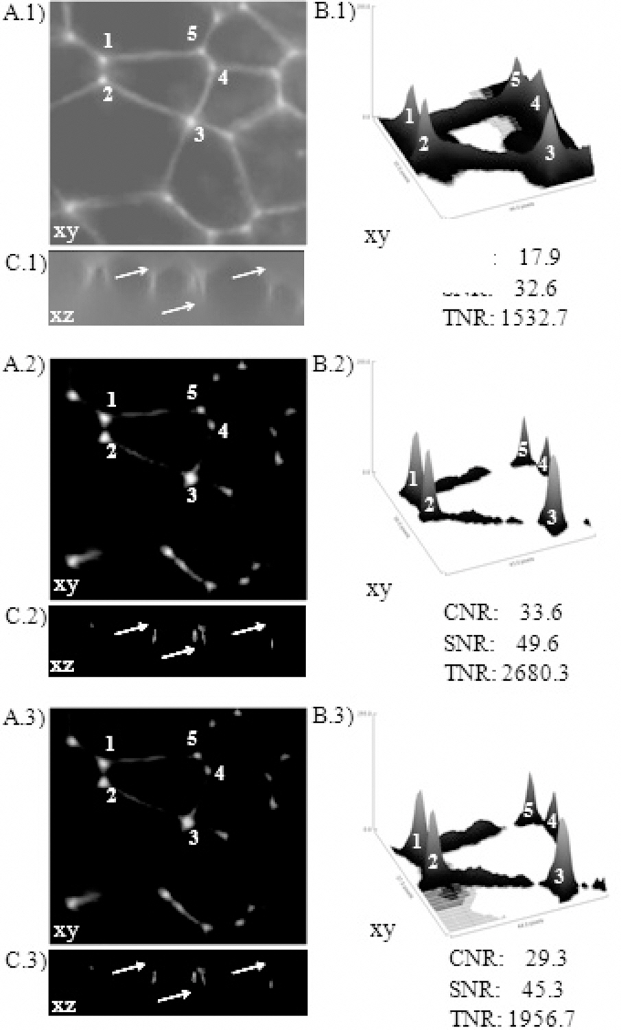
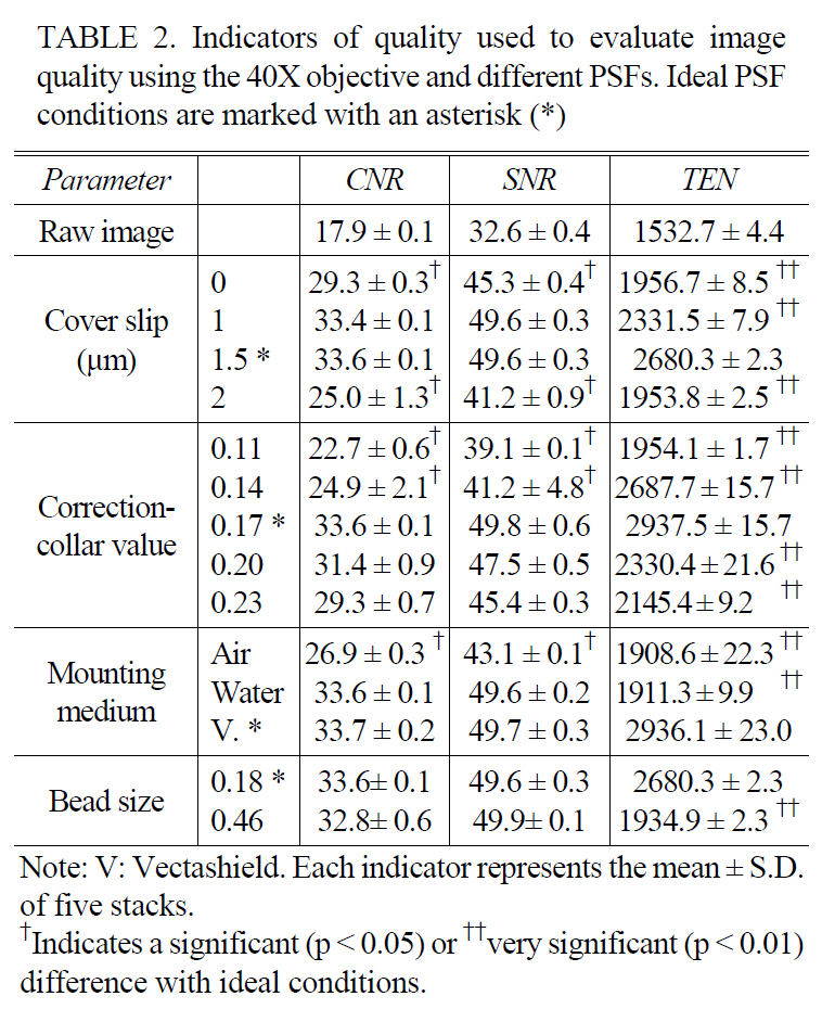
Figure 5 (40X objective, stack of 256 × 256 × 128 pixels3)and Table 2 show the results of deconvolution experiments using different PSFs. In the figure, row 1 represents raw images, row 2 is row 1 after deconvolution using an ideal PSF, and row 3 is row 1 after deconvolution with a nonideal PSF. To compare the improvements introduced by deconvolution, we used three representations: set A shows maximum-intensity projections, set B the surface plot of five points indicate in set A and set C one axial cross-section(x-z plane).
Qualitatively, in set A we note a better contrast in the points (cell-cell contact), higher intensities in the surface plot (set B, numbers) and in set C the axial asymmetry was removed (arrow). Quantitatively, we used the image-quality indicators CNR, SNR and TEN; all of them present higher values after deconvolution. Working with the 40X objective,the indicators were: 17.9 ± 0.1, 32.6 ± 0.4 and 1532.7 ±4.4 (raw image); 33.6 ± 0.1, 49.6 ± 0.3, and 2680.3 ± 2.3(deconvolution using an ideal PSF); and 29.3 ± 0.3, 45.3± 0.4, and 1956.7 ± 8.5 (deconvolution a non-ideal PSF).With the 100X objective (data not show), the indicators were: 17.4 ± 0.6, 32.9 ± 0.4, and 1124.9 ± 3.5 (raw image);
24.1 ± 0.1, 40.1 ± 0.2, and 1690.9 ± 4.7 (deconvolution using an ideal PSF); and 24.1 ± 0.1, 40.1 ± 0.01, and 1687.8 ± 5.5 (deconvolution using a non-ideal PSF).
In both cases (40X and 100X), image-quality is improved very significantly after deconvolution; but if we compare deconvolution outcomes, changes in general are not significant between CNR and SNR, but are significant or very significant between TEN and CNR, and TEN and SNR, respectively.Moreover, image-quality after restoration using an ideal PSF was always the highest (Table 2).

Indicators of quality used to evaluate imagequality using the 40X objective and different PSFs. Ideal PSFconditions are marked with an asterisk (*)
It has been previously demonstrated that the image formation process in 3D microscopy (such as the system used in this study) differs from classical image formation theory [9].Moreover, it is very well known that the accuracy and quality of the PSF are essential to ensure the correct outcome of any deconvolution process. Therefore, the main purpose of our experiments was to evaluate suitable imaging conditions to correctly obtain a PSF and to discuss how variations on these conditions affect deconvolved images. According to our knowledge, several authors studied the first set of mentioned problems [2]; [4-5]; [9, 12], however there are few works that quantitatively evaluate the latter aspect of this approach [11].
To obtain a correct determination of a microscope’s PSF,it is advisable to measure the PSF under the same conditions as the sample itself [9]. Good results are obtained if the PSF is obtained directly inside the biological objects (e.g.,by injecting fluorescent beads). Since this task was difficult to apply because of the highly pigmented
Under these conditions, we demonstrated that PSFs resemble the ideal one and has axial symmetry (though a small elongation was observed) and reflection symmetry about the focal plane (Figure 2); indicating the good quality of our lenses.This was not surprising because modern microscope optics are highly sophisticated and are corrected to high levels of precision to avoid distortions [20]; and fundamentally because microspheres were imaged just below the cover slip. In Figure 2, it is also possible to analyze the importance of microsphere size in the determination of the PSF. The selected bead should be as small as possible (below to the resolution limit of the microscope). We showed that bigger beads present larger FWHM values (1.85 ㎛ to 0.46 ㎛ diameter) compared to smaller beads (1.54 ㎛ to 0.18 ㎛ diameter) for the same objective. Similar results were found in previous works using Olympus Plan-Apochromat 63X/1.4 oil objective, where FWHM values grow with increasing bead diameter (1.02 ㎛ to 0.1 ㎛ diameter, 1.10 ㎛ to 0.20 ㎛ diameter, and 1.4 ㎛ to 0.5 ㎛ diameter) [12].The dependence of FWHM on object size approaches linear behavior for large bead diameters. We also noted that poor restoration is achieved when using beads with diameters larger than the resolution limit, (Table 2).
When we performed variations in the previously defined optical path, PSFs fundamentally exhibit an axial asymmetry that resulted in light dispersion and hence in a loss of resolution (higher FWHM values) (Figure 3). These variations produce alterations in the optimal path for which the objectives were designed and appears when the conditions of observation differ from the ideal one [22-23], resulting in spherical aberrations [6-9]. These results coincide with those of previous works. Kozubek work has demonstrated that the intensity peak of the PSF decreased and a significant increase of the FWHM in the axial direction (dZ) appeared when he evaluated variations with different embedding medium(FWHM was approximately 1.15 ㎛ and 1.20 ㎛ for immersion oil and water respectively), with cover slip thickness (discussed below) and also with beads located at different depths(FWHM was approximately 1.11 ㎛, 1.28 ㎛ and 1.4 ㎛ to 1 ㎛, 4 ㎛ and 10 ㎛ below the cover slip, respectively)[12]. Likewise, Keller and coworkers have shown a decrease in PSF intensity distribution when they evaluated cover slip thickness (around 30% and 50% from the ideal one using 150 ㎛ and 130 ㎛ thickness, respectively). Also,they have demonstrated that Plan Apochromat objectives (like our lens setup) have the best intensity distribution compared to Plan-Neofluar and Achromat objectives, confirming the quality of the lens [7].
We find a similar behavior in the two lenses tested, however since the axial resolution of a fluorescence microscope is proportional to η/(NA)2, a dry lens has significantly worse axial resolution (Figure 3B) if compared with an oil-immersion lens (Figure 3D). In our case, the dry 40X lens (NA 0.85)has a z-resolution 1.6 times worse than oil-immersion 100X lens (NA 1.35). This is important because usually many researchers use dry objective lenses to achieve a long working distance or to avoid the mess of using oil. Therefore,according to previous data, the ratio of the two refractive indices determines how important the effects of spherical aberration become. The NA is preserved in the transition from one medium to the other, and the NA in the medium is therefore also close to 1.
Other important point to consider is that the vast majority of existing dry objectives are corrected for 170 ㎛-thick cover slips (N° 1.5). Since considerable variability exists even among cover slips of a given number, precise knowledge of cover slip thickness is critical. In our experiments the best imaging results (lower FWHM, higher CNR, SNR, and TEN values) were obtained using 170 ㎛-thick cover slips(Figure 3A, 3B) and employing a correction value of 0.17.FWHM was 1.51 ㎛ for the optimal condition (170 ㎛),and 3.36 ㎛, 1.92 ㎛, and 2.68 ㎛ for 110 ㎛ 150 ㎛,and 210 ㎛ thicknesses, respectively. Similar behaviors have been demonstrated in other works. Keller, using Plan-Neofluar 63X, NA 1.2 water objective, has obtained an FWHM of 0,70 ㎛ for the optimal condition (170 ㎛),and 2.00 ㎛, 2.50 ㎛, and 1.30 ㎛ for 150 ㎛, 120 ㎛,210 ㎛ thicknesses, respectively [7]. Therefore, with tolerance of ± 10 ㎛ for top-quality cover slips, the FWHM changes by more than a factor of 2. With increasing NA (> 0.5),particularly with dry and water immersion leses, selection of cover slip for correct thickness is particularly important.Even oil-immersion lenses perform optimally only with a cover slip thickness of 170 ㎛. Kozubek, using Plan-Apochromat 63X, NA 1.4 oil objective, has obtained a FWHM of 1.10 ㎛ for the optimal condition (170 ㎛), and 1.14㎛, and 1.16 ㎛ for 140 ㎛, and 100 ㎛ thicknesses,respectively [12].
Regarding oil-immersion lenses and in accordance to previous reports [4, 9], we obtained an optimal optical path using oil with η ? 1.516 (Figure 3C, 3D). Scalettar et al [11] demonstrated that oils with higher or lower η yield positive or negative optical path length errors. We obtained similar results when testing lower refractive indices. FWHM was 0.90 ㎛ for the optimal condition (Olympus oil, η=1.516), and 1.12 ㎛, 1.40 ㎛, and 2.60 ㎛ for glycerol(η=1.47), water (η=1.33), and air (η=1.00), respectively [23].Therefore, with oil-immersion objectives, it is recommended to obtain the immersion oil from same company that manufactures the objective lens.
In summary, a positive optical path length error yields a PSF with excess intensity in sections collected when the lens is furthest from the cover slip, whereas a negative optical path length error yields a PSF with excess intensity in sections collected when the lens is closest to the cover slip.
To evaluate how previous conditions affect the deconvolution process, we first used 4 ㎛ fluorescent beads as pattern specimen. Since the exact size of these was known, we could use the FWHM parameter to measure their diameter, and therefore assess the quality of restoration after deconvolution by measuring the reduction in z-axis elongation. From diffraction-limited effects and constraints imposed by geometrical optics, the image of real beads becomes elongated in the z-axis and unprocessed bead images present a diameter of 6.3 ㎛ (by FWHM). Optimal restoration (in order to obtain the real shape), as has been noted previously [10],is impossible. However, this elongation was reduced to about the real diameter (4.12 ㎛) when deconvolution was carried out using an ideal PSF (Figure 4). As expected, when we changed the PSF to a non-ideal one, poor restoration was achieved, evidenced by higher FWHM values. As opposed to an ideal PSF, asymmetric PSFs introduce artifacts in deconvolved images showing a lower reduction in the elongation (significant). Additionally, a small change in the refractive index of mounting medium from η=1.47(Vectashield) to η=1.46 (glycerol), showed the highest value of FWHM (very significant) indicating the effects of the altered optimal optical path.
In order to assess restoration changes in a biological specimen, we used Rhinella arenarum embryo images. This biological specimen is very complex and contains significant refractive index heterogeneities. A similar complexity would be found if we worked using live cell microscopy. In these cases, where mismatch is significant, it may result in the PSF becoming non stationary, especially along the axial direction [24-25]. Effectively, we have found that embryo raw images present spherical aberrations (Figure 5 set C, x-z plane). Therefore, it was difficult to implement the same optical setup for the PSF determination. In this mismatched setup, the only part of the specimen that can be observed without the severe effects described above is the one immediately below the cover slip. Therefore, a locally defined PSF is unlikely to remove the effects of spherical aberration using a global deconvolution. However,there is evidence suggesting that high-quality deconvolution of images of thick objects can be achieved without introducing this complexity into the deconvolution algorithm [11, 26].In our lab, we have recently obtained similar images, using setups that are up to 25 ㎛ below the cover slip [17].These images have been very well deconvolved despite the considerable distance between the object and cover slip.
We have demonstrated that, for all processed images presented, deconvolution with our empirical PSF clearly improves image quality (numbers and arrows in Figure 5).It enhanced contrast and decreased blurring, mainly in the axial direction (arrows). Such an improvement should always occur, providing that the PSF estimate used is correct. Even planes distant from the cover slip, for which we know the PSF is not perfectly valid, do not present strong artifacts.
However, to get the best performance in live cell microscopy,or when thick specimens are used, it is necessary to predict the axial broadening variation of the PSF dependant on the depth of the sample [27]. This has been measured using subresolution beads either embedded in optical cement[10] or fixed to a tilted surface [28]. However, both of these measurements use beads placed at random depths to measure this effect. Because the depth is not changed systematically in these experiments, one must interpolate between the measured PSFs to use them for 3D deconvolution[21]. Recently, to resolve this problem, Shaevitz and Fletcher,have designed a system in which the depth variant PSF could be measured systematically and quickly with a single bead in any liquid medium [29].
In this work, it was very difficult to qualitatively determinate the best deconvolved image. Deconvolved stacks (Figure 5) look very similar in any representation (row 2 and row 3). Therefore, to determine which PSF works better for deconvolution, a quantitative evaluation is necessary. Previous work from Sibarita has measured only intensity profiles and added arrows (over three optical sections and one axial cross section) to illustrate the improvements in CNR and SNR ratios [9]. Similarly, we found improved CNR and SNR ratio values in deconvolved images using an ideal PSF and an aberrant one if compared to unprocessed stacks. However,if we compare processed stacks among themselves, these indicators in general do not show significant variations in almost all PSFs tested. Since CNR and SNR do not show significant differences, we selected another parameter that is currently used to automatically determine the best focal plane [18, 30], assessing image clarity, namely TEN. Using this indicator we demonstrated that significant differences exist between deconvolved images when the PSFs employed are not ideal (Table 2). According to our data we conclude that PSFs obtained under conditions similar to those of the specimen yield better processed images. Moreover, images collected under non-optimal imaging conditions will exhibit some degree of spherical aberration; these images should be deconvolved with a PSF with similar degree of spherical aberration.
results are obtained when the empirical PSF utilized is obtained under the same conditions as the specimen. Therefore, we need a relatively small library of PSFs that spans common types of image aberrations, which will suffice for high quality deconvolution of most images. We also demonstrated that it is very important to quantitatively check the process’outcome using several quality indicators. We detected a significant improvement when using an indicator to measure the focus of the whole stack. Therefore, one approach that we are pursuing is to use TEN indicators to develop a scheme for automatically choosing the optimal member of library by performing three trial deconvolutions at reduced resolution. From this, the best PSF could then be chosen for more extensive deconvolution at full resolution. Another solution is to use an automatic algorithm recently developed for us [31]. It took around three hours to complete an image processing task similar to the one we used in this paper,to deconvolve each of two raw 3D images (40x and 100x)with all different PSFs (thirty experimental conditions, n= 5), that is over 250 different deconvolution processes,followed by the evaluation of the resulting deconvolved images with the TEN indicator. Since an image obtained from any microscope (such as wide-field, confocal or twophoton)can be further improved by deconvolution, we believe that it is fundamental to use these quantitative indicators.
In the future we will be considering the effects of depth variation and noise suppression in the empirical PSF. Others authors have already determined the PSF considering these factors and demonstrated that it is possible to obtain an additional improvement in deconvolved image quality [29,32]. Moreover, recent new approaches are utilizing PSFs calculated in amplitude and phase [33].

![Schema of the optical setup in an upright microscope.Ideal (left) and real (right) situations are compared. Beadsstained with fluorescent dyes [white circles (3)] are attached tothe surface of a microscope slide (5) covered with an mountingmedium (4) covered with a cover slip (2) and observed throughthe immersion oil (1) using an oil-immersion objective (100X).](http://oak.go.kr/repository/journal/10727/E1OSAB_2011_v15n3_252_f001.jpg)