Recently much research and many inventions for the development of laser scanning optical systems have been carried out in order to improve their resolution in keeping with the increase in the use of computers in a modern society. The greater part of the results are published in patents[1-11]and in books,[12-14] but these works need more general and theoretical analyses.

The goal of this paper is to theoretically and synthetically analyze the distortion, spot size and field curvature required for a laser printer system in order to get a smaller and more uniform spot size. Also, we show theoretically how to minimize of the radius of the rotator by adjustment of the entrance pupil position in order to make a more compact laser printer.

A general type of laser printer consists of a semiconductor laser as a source, a collimator lens, a rotating mirror (in general a polygonal mirror), and a so-called "f-θ” lens. The laser beam, assumed to be Gaussian, passes first through a collimator, and the parallel beam that is formed by the collimator makes a spot on a recording plane after passing through the polygonal mirror and the “f-θ” lens. All elements are important, but the "f-θ” lens is the most complicated and main part of the laser scanning optical system.

When we design the “f-θ” lens, two important things are considered: (1) the movement of the light spots cast on a recording plane by a polygon with a constant angular velocity has to be proportional to a scan angle, i.e. y' =f?θ, where y' is the image height, f is the focal length of the “f-θ” lens and θ is the scan angle. In order to solve this problem we will define the “f-θ” distortion and investigate its allowable and optimum values. (2) The sizes of these spots must be uniform on the recording plane. The spot size is primarily determined by field curvature in practice, so we will investigate the tolerance of field curvature with the analysis of binary spot size and the Gaussian beam property. These topics will addressed in detail, and we will analyze not only the properties of these aberrations but also their allowable values.

Note that other aberrations such as spherical aberration and coma, etc., can be disregarded due to the small aperture of the beam passing through the “f-θ” lens. The effect of these aberrations will be discussed in the section 4.

When the polygonal mirror rotates, as is known, the entrance pupil position travels along the scan angle θ in the laser printer system[12, 15]. (In general we put the entrance pupil position on the facet of the rotator.) The smaller the size of the rotator, the smaller the change of entrance pupil position and the more compact the laser printer system. In order to minimize the size of the rotator we will introduce the shifting angle of the input beam along the facet of the rotator. Thus, the minimum size of the rotator and the changing value of the entrance pupil position will be derived without approximation.

In order to reduce the influence of errors introduced in the manufacture of the rotator on the image shift in the perpendicular section of the recording plane, i.e. in the sagittal section, we can choose an optical system in which the sagittal section is different from the meridional. However, in this paper we will limit our analysis to the meridional section.

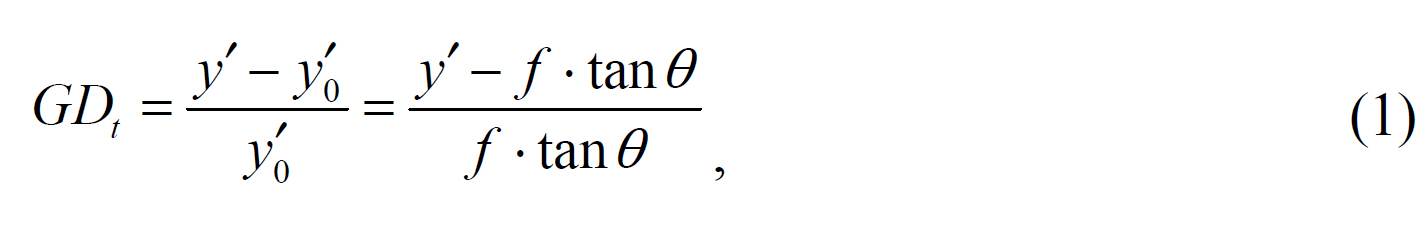
An ordinary distortion-free lens has the image height which follows the rule y₀'=f?tanθ, where y₀' is the ideal image height. Therefore, as is known, a common fractional distortion GD_t is usually calculated from the following equation[15]:

where y' is the actual image height formed by a chief ray.

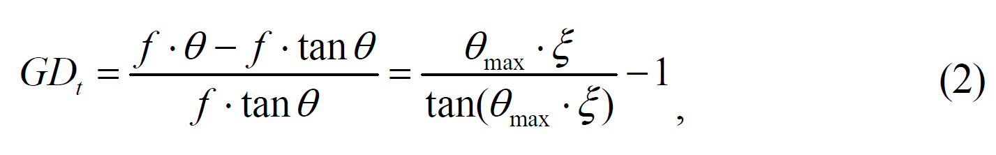
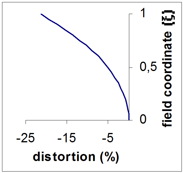
In the case of a perfect “f-θ” lens, i.e. y'=f?θ, from Eq.(1) we have the following common fractional global distortion:

where ξ=θ/θ_max (0≤ ξ ≤1) is a fractional field coordinate. The plot of this distortion versus ξ is shown on Fig. 1 (in the case of θ_max=45°).

According to the general Eq.(1) the distortion of the “f-θ” lens must have a large negative value (large barrel distortion). Therefore, during the design of the “f-θ” lens we have to introduce a large controlled distortion value along the curve shown in Fig. 1, but it is very inconvenient to do so.

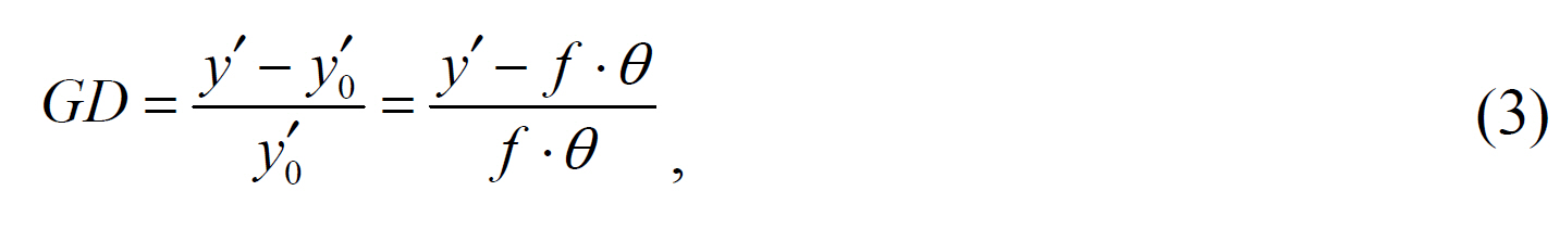
The alternative way is to use a lens design program which is able to calculate distortion by using y₀'=f?θ rather than y₀'=f?tanθ. In this case the fractional distortion called the global “f-θ” distortion has the following form:

When we use the global “f-θ” distortion Eq.(3) instead of Eq.(1), the distortion of the “f-θ” lens system does not need to be corrected with a large negative value and simply must have the smallest value available. The global “f-θ”distortion will be called global distortion in this paper.

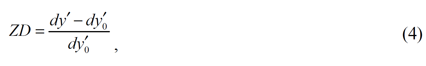
Let us investigate the distortion of the “f-θ” lens in detail. Many authors use the so-called calibrated focal length, instead of the paraxial focal length, to reduce maximum global distortion in the “f-θ” lens[12]. But in order to obtain the optimal form of the correction and the tolerance of distortion in the laser printer system, we must note that the distortion has to be considered as non-uniform velocity of the scanning spot, i.e. as non-uniformity of the sizes of the groups consisting of several spots on the recording plane. This indicates that we have to consider not the global distortion according to Eq.(3) but local or zonal distortion(ZD), which is determined as change not in y' but in the differential of y' as follows:

where dy' and dy0' are the differential heights of y' and y0' corresponding to differential scan angle dθ, respectively.

Only the ZD is important for the design and evaluation of the laser scanning system and the proper specification must be done for its value. The question is what value of ZD must be considered. The simple analysis shows that we must use not the maximum value of ZD but its peak-valley value (the difference between maximum and minimum value). If we use ZD during the design of the “f-θ” lens, we only have to minimize the peak-valley value of ZD.However, the problem is that ZD is not convenient for optical designers, who commonly use GD according to Eq.(3).Also, all commercial computer programs for optical system design use GD. In fact, when we use GD, it is not enough to minimize its value; it is very important to have the optimum form of distortion curve. To solve this problem we will determine the relation between GD and ZD. From Eqs.(3) and (4) it is easy to find the relation of these distortions as follows:

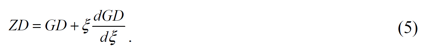
In general, as it is enough to consider only the 3rd and 5th order distortion for the “f-θ” lens, we can write GD as follows:

where a and b are the coefficients of the 3rd and 5th order distortions, u=ξ². From Eqs.(5) and (6) ZD is expressed as follows:

With the factor Κ=a/b we can express Eqs.(6) and (7) as follows:

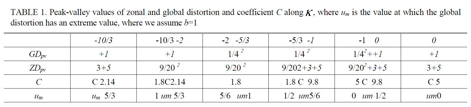
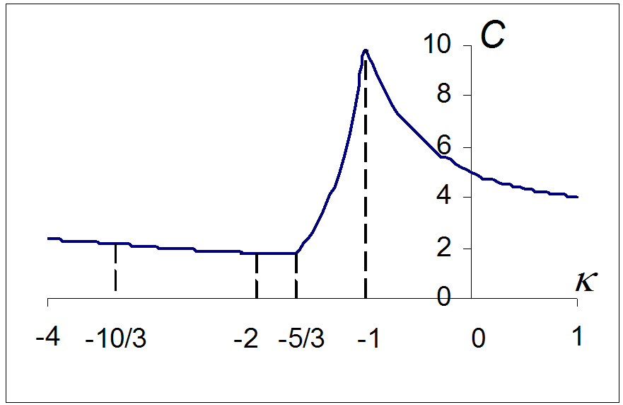
The factor Κ shows the relation between the 3rd and 5th order distortions, hence it determines the form of the distortion curve. Our task is to find the optimal value of Κ, i.e. the optimal form of global distortion correction. To complete this task, we introduce the coefficient C=ZD_p-v/GD_p-v in the ratio of the peak-valley value of ZD to GD. It is clear that the smaller the value of coefficient C, the better the form of the distortion correction. Table 1. shows the peak-valley values of ZD and GD along Κ, and Fig. 2 shows the plot C versus Κ, all from Eqs.(8a) and (8b).

In Fig. 2 we can divide Κ into two regions with boundary at Κ=-5/3. The coefficient C shows a comparatively gradual slope and a small value in the range Κ ≤-5/3. A sharp slope and large value in the range, Κ >-5/3, characterizes coefficient C. Thus, the former is a good region for the correction of ZD and the latter is inferior. In particular, in the best case the coefficient C has a minimum value 1.8 in the range -2< Κ <-5/3, but in the worst case C has a maximum value 9.8 at Κ=-1. For example, if GD_p-v is 0.2% and Κ=-1, then C=9.8 and ZD_p-v is obtained 1.96%(ZD_p-v=C?GD_p-v). That is even worse than the case of GD_p-v=0.5% and Κ=-5/3 ( (ZD_p-v=0.9%). If Κ=±infinity, we have only 3rd order distortion and in this case from Table 1, we see C=3.

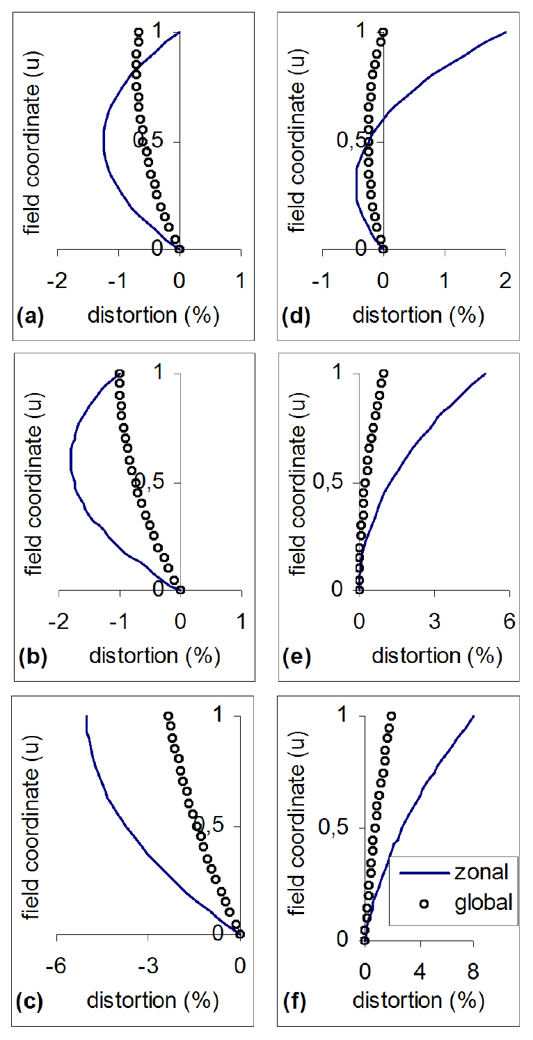
During the design of an “f-θ” lens we have to know the value C or Κ for the correction of ZD. Its value can be obtained from the shape of GD because it depends on the value u_m, and this value u_m is decided by the factor Κ (u_m=- Κ/2). The value u_m along Κ is given in Table 1 and Fig. 3 shows the shapes of GD and ZD along various Κ.

In order to obtain a satisfactory ZD of the “f-θ” lens we suggest the shape of GD must have the forms (a), (b)or (c), in the left parts of Fig. 3, and must avoid the forms (d), (e) and (f), in the right parts of Fig. 3.

Ultimately, we have to consider not only the value of GD, but also its shape for the correction of ZD during the design of the “f-θ” lens.

Note that from our analysis the calibrated focal length that is used to reduce the maximum value of GD[12] cannot reduce the peak-valley value of ZD.

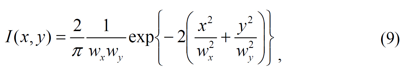
From the theory of Gaussian beams[16] the normalized irradiance of a Gaussian beam is expressed by the following form in any plane:

where w_x and w_y are the beam radii at which the irradiance is exp(-2) of the maximum value in x and y coordinates respectively, i.e. the beam has 86.5% of total beam power in the beam radius (w_x ²+w_y ²)^1/2 from properties of Gaussian function. Let us focus on the meridional section only, i.e.x=0.

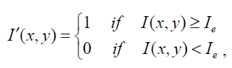
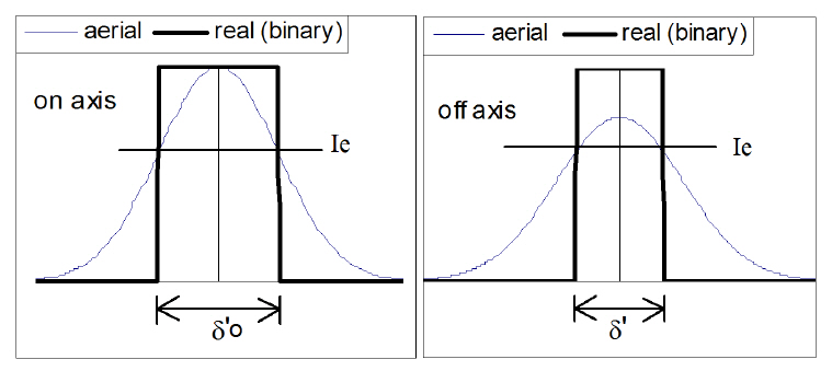
The analysis of spot size on the image plane depends on the kind of scanning system. If any system is used to scan an image for computer image processing, we have to analyze the aerial spot image and evaluate the spot size at the level of beam power 86.5%. For more detailed analysis in this situation we have to use MTF of scanning system. Nevertheless, our consideration deals with the laser printer and laser processing scanning systems. Such systems, laser printer and laser cutting device and so on, are characterized as the non-linear process of spot image detection. If the exposure is higher than a reference level I_e (I> I_e), it is recognized as a white image (for the printer) or cut material(for the cutting device) but if I< I_e, then it is black or fails to cut This image transformation may be called binary according to the following equation:

where I(x, y) is the aerial image and I'(x, y) is the detected(binary) image. (See Fig. 4).

For such a process the use of MTF is not proper and the binary spot size has to be determined in a different manner from the aerial image.

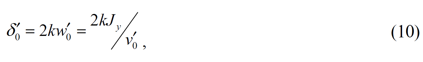
The binary spot size for on-axis beam in meridional section can be expressed as follows on the recording plane:

where δ₀' is the binary spot size of on-axis beam on the recording plane in the meridional section, v₀' is the angular beam divergence in the image space and can be considered as the exit numerical aperture A₀' of the “f-θ ” lens, w₀' is the beam radius at which the irradiance is exp(-2) of the maximum value on the recording plane, J_y is Lagrange invariant in the meridional section and k is a coefficient to depend on I_e. Here we assume the beam waist on-axis is located on the recording plane. For example, in the case of I_e=I₀exp(-1/2),then k is 0.5, where I₀ is the maximum irradiance of the on-axis beam.

In general, since every laser does not have perfect coherence, we must consider Lagrange invariance in deciding the spot size of the Gaussian beam. Therefore, Eq.(10) is a more general equation than the known equation δ₀'=aFλ[13], where a is the aperture shape factor, F is the F number and λ is the wavelength.

The value k which decides the binary spot size may be arbitrarily chosen, but we must select the optimum value k. We suggest k=0.5, and in this case I_e=I₀exp(-1/2) is put at the point where the Gaussian curve has a maximum slope. It indicates that the non-uniformity of the binary spot sizes is very small on the recording plane under an instability of the reference irradiance I_e. Also, the effective binary spot size is two times less than in the case of I_e=I₀exp(-2) or k=1.

In the case of off-axis, the beam radius w' on the recording plane is larger than w₀' in spite of the fact that total beam energy is conserved, so the maximum irradiance is smaller than it is in the case of the on-axis (see Fig. 4). On the other hand, since the reference irradiance I_e is fixed, the binary image size of off-axis differs from that of the on-axis. In order to know how the binary image size of off-axis changes, let us introduce two parameters η and γ:

where η and γ are the fractional changes of aerial spot radii and binary spot radii respectively, which are determined by an arbitrary reference irradiance I_e. w₀' and w' are the Gaussian beam radii of the on-axis and the off-axis respectively, that contain 86.5% of beam power (aerial spot radii). Also w_b0' and w'_b are the binary spot radii of the on-axis and the off-axis beam with a defined power respectively, and w_b0'=k_w0' from Eq.(10). In fact, from the parameters η and γ we can see the non-uniformity of aerial and binary spot size during the movement of the scanning spot on the recording plane.

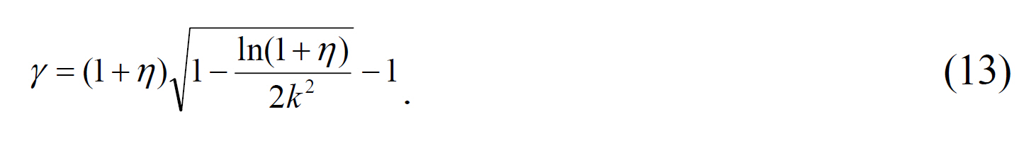
From Eqs.(11) and (12) and with the relation between the reference level Ie and the Gaussian curve of off-axis, i.e. exp(-2k²)/w'₀=exp{-2(w'_b/w')²}/w', we obtain γ as follows:

For a small η, i.e. η<<1, for the case of k=0.5 Eq.(13) is approximately expressed as follows:

From the negative sign of Eq.(14) we see the binary spot size of the off-axis beam is always smaller than that of the on-axis (since w_b'=w₀'(1-η²)) and the change of the off-axis spot size is proportional to the square of a small value η. For example, if η=20%, then γ=4% according to both Eq.(13) and Eq.(14). If η =40%, then γ=20% from Eq.(13) and γ=16% according to simple Eq.(14). From the above example we can use the simple Eq.(14) as an approximation for the case of η<40%. For a greater η we can reduce the value γ by the choice of the proper value k from Eq.(13). It is interesting to note from Eq.(14) the binary process of detection favors spot size uniformity better than other processes, and with the binary detection we have greater tolerance for aberration.

In the result, when we choose k=0.5 the change of the off-axis binary spot size has the small value under the change of the off-axis Gaussian beam envelope, and the change of the on-axis binary spot size Δδ₀' has a minimum value under an irradiance instability ΔI_e.

In addition, the length l of scanning line on the recording plane is expressed as follows:

Also the exit numerical aperture A₀' of the “f-θ ” lens is connected with the focal length f of the “f-θ ” lens and the incident parallel beam diameter D:

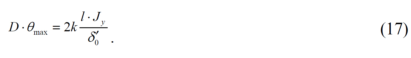
From Eqs.(10), (15) and (16) we have the following relation:

The parameters of the right hand side of Eq.(17) (the length of scanning line, Lagrange invariant of a laser beam and spot size on a recording plane) are already given. The parameters of the left hand side (the beam diameter and the maximum scan angle) can be arbitrarily chosen under the condition of a constant preservation of their product. Lagrange invariant depends on the quality of the laser beam, and for the perfect beam we have the minimum λ/π. For example, in the case of 1200 dpi. δ₀'=21.2 ㎛, l=220 mm, J_y=λ/π (λ=7800A), k=0.5 and θ_max=45°, from Eq.(17) we can easily ascertain a beam diameter of D=3.28 mm., but if we choose J_y=λ, then D=10.3 mm. We can see the quality of laser beam (degree of coherence) is very important in a laser printer system because the smaller the beam diameter, the better the resolution of a printed image.

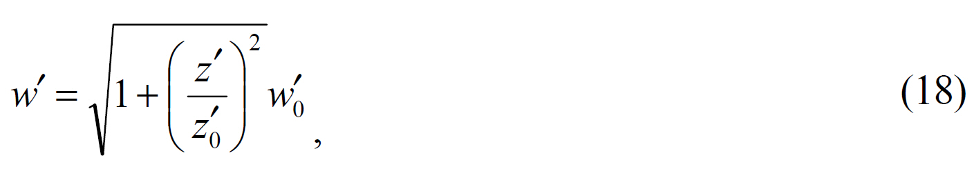
Now we consider the requirements for the correction of a meridional field curvature within an allowable non-uniformity of spot sizes on the recording plane. From the fact that the laser beam has Gaussian beam properties, the beam radius is decided by the following form both in meridional and sagittal section on the recording plane:[16]

where w' is the beam radius on the recording plane, w₀' is the beam radius in the waist, z' is the distance from the recording plane to the beam waist, and z'₀=w₀'/v₀'=w₀'²/J is the Rayleigh range. In this section we assume that the beam waist radius of the off-axis is equal to that of the on-axis since we want to see the effect of the variation of spot size due only to the meridional field curvature. For analysis in the meridional section, we use z'_m and J_y instead of z' and J in Eq.(18) respectively, where z'_m is the meridional field curvature and J_y is the meridional Lagrange invariant.

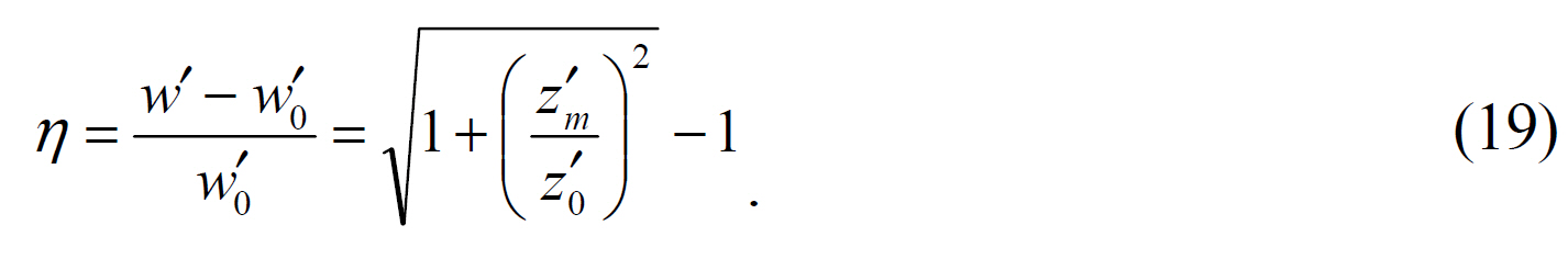
The fractional non-uniformity of the aerial spot sizes due to the meridional field curvature is defined by the following expression from Eqs.(11) and (18):

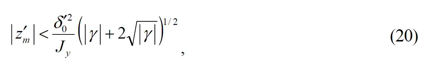
From Eq.(14) and δ₀'=w₀' (in the case of k=0.5) we can determine a tolerance limit of a meridional field curvature:

where γ is an allowable fractional non-uniformity of binary spot sizes. For example, in the case of γ=10%, δ₀'=21.2㎛ (1200dpi) and J_y=λ/π (λ=7800A), then z'_m<1.55 mm but in the case of J_y=λ we have z'_m<0.49 mm. Eq.(20) as well as Eq.(14) are comparatively accurate in the case of small η. However, if η is larger than 0.4, we cannot get a simple expression and the problem may be solved by numerical analysis. We limit our analysis only to small values of η.

In fact, we have to use w'/cosθ' instead of w' in Eq.(19) since the direction of the off-axis outgoing beam is not consistent with the normal direction of the image plane, where θ' is the angle between a chief ray and an optical axis in the image space. In this case z'_m (the tolerance limit of meridional field curvature) is expressed as follows:

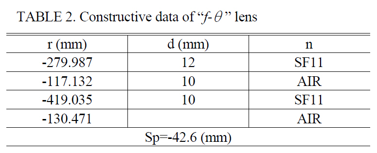
Let us consider an example of the design of a simple“f-θ” lens according to the previous analysis of distortion and meridional field curvature z'_m (in section 2 and 4):

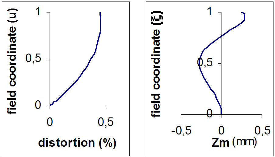
Table 2. shows the parameters of “f-θ” lens: r is the radius of curvature, d is the corresponding axial distance, n is the name of the glass as given in the Shott catalog and S_p is the entrance pupil position, i.e. the distance between a center of the rotator facet (in the case θ=0) and a first surface of the “f-θ” lens. We designed this system with two spherical lenses so that the non-uniformity of the spot movements(ZD) and the meridional field curvature do not exceed 1%and 0.3 mm respectively (see Fig. 5).

In addition, let us investigate the influence of coma in the “f-θ” lens on the spot position. In the case of the above preliminary “f-θ” lens the maximum value of coma is about 0.0325 mm for the beam diameter of 10 mm at the end of the field, and the shift of the effective spot center due to this effect is less than 0.0325 mm. In fact, the shift of an effective spot center is 0.0074 mm according to wave front criterion (minimum RMS wave front deformation) and 0.0111 mm according to geometrical criterion (minimum RMS transverse aberration). When we compare these values with GD (-0.459 mm) at the end of a field, we can neglect the effect of coma. In general, the effect of coma can be disregarded in the system with the small aperture.

In order to minimize the change of an entrance pupil position and to make a compact system, it is very important to minimize the radius of the rotator. But, it is impossible to have an extremely small size of rotator because the radius depends on the input beam diameter D.

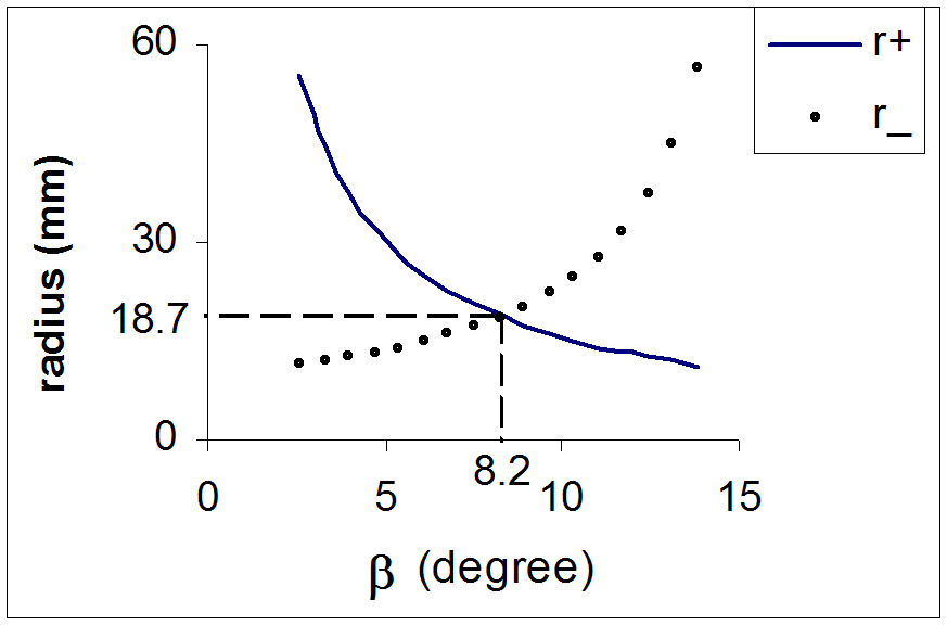
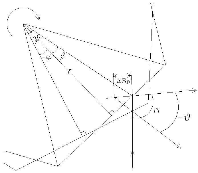
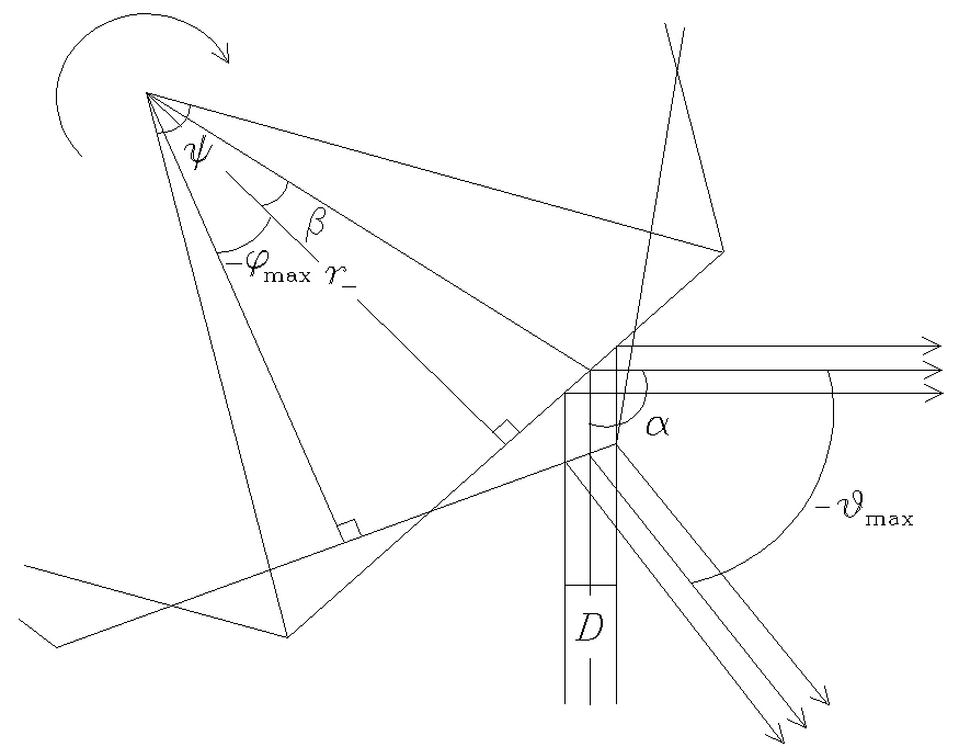
We want to find the minimum radius of rotator under the given conditions: a maximum scan angle θ_max, a vertical angle of rotator ψ =π/n (where n is the number of rotator facets), a shifting angle β of the incident chief ray from the center of the rotator facet along the facet in the case of θ=0, the incident beam width D, and a variation angle α of optical axis direction in the case of θ=0. From the geometry in Fig. 6 we can find the minimum radii of rotator r₊ and r_- at which the incident beam reflects from the mirror of rotator without losing it, where r₊, r_- are the minimum radii of rotator when the polygonal mirror rotates counterclockwise and clockwise respectively:

From Eq.(22) we can see the smaller β, the larger r₊ and the smaller r_-, but the size of rotator is determined by the greater value of r₊ and r_- (see Fig. 7).

In the case β=0, r₊ is always larger than r_- and the radius of rotator has to be chosen as r₊. From Fig. 7 we can see that the radius of rotator has a minimum value when r₊ is equal to r_- and in this case tanβ can be expressed by the following form:

From Eqs.(22) and (23) we can get a minimum radius r:

Of course, the smaller the α, the r, i.e. we can reduce the radius of the rotator by the proper choice of parameters.

In a design process, it is assumed that the direction of the incident beam changes centering around one fixed point on the rotator facet, therefore the entrance pupil position is usually located at this point. In general, the entrance pupil’s position is fixed at an intersection point between a chief ray and an optical axis in an optical system. However, in the “f-θ” lens the entrance pupil position cannot be constant and identical to all field coordinates because of the geometry of beams deflected by the rotating polygonal mirror[12, 15]. So, we must consider the fact that the entrance pupil position of the “f-θ” lens is changed by the rotating polygonal mirror in the real laser scanning system (see Fig. 8).

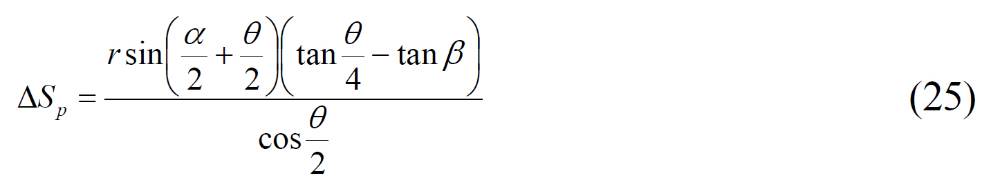
From Fig. 8 the change of the entrance pupil position ΔS_p can be exactly expressed by the following form:

where r is the perpendicular distance from the center of the rotator to its facet, and θ is the scan angle. Here the scan angle θ is positive if the polygonal mirror rotates counterclockwise, and negative if it rotates clockwise.

From the introduction of the angle β we can very effectively reduce not only the radius of the rotator but also ΔS_p. For example, when D=10 mm, θ_max=45°, ψ=60° and α=45°,if we introduce β of Eq.(23), then β is 3.43°. In this case, the minimum radius r is 35.91 mm and ΔS_p changes from -1.18 mm to 3.82 mm, but if β=0, then r=59.65 mm and ΔS_p changes from -1.17 mm to 5.46 mm.

Note that Eqs.(22), (23), (24) and (25) are derived for the general case and without any approximation.

We have shown that the distortion in the “f-θ” lens should be evaluated with the peak-valley value of ZD instead of the maximum value of GD. We derived how to correct ZD of the “f-θ” lens with the relation between the 3rd and 5th order distortion and the ratio of the peak-valley value of ZD to GD. Also, we focused on the importance of the form of the global distortion curve and suggested several good forms for the correction of ZD in the “f-θ” lens.

The spot size that is detected on the recording plane of a laser scanning system was analyzed not by aerial image but by binary image, and we have pointed out that the reference irradiance for binary image has to be selected as I_e=I₀exp(-1/2), i.e. k=0.5 when the change of the aerial spot size η is comparatively small.

In order to decide a tolerance limit of meridional field curvature we utilized the analysis on the change of the binary spot size and the Gaussian beam properties. From these tools we obtained the general forms of Eqs.(20) and (21).

We know that the smaller the radius of the rotator in a laser printer system, the smaller the ΔS_p and the more compact the system size. Therefore, it is natural that the radius of the rotator must be as small as possible. From Eqs.(23) and (24) we may always find the minimum radius of the rotator.