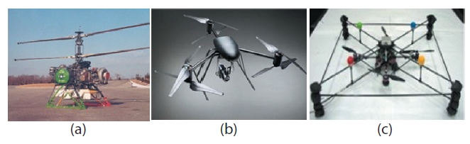
Recently, the significance of the small-size unmanned aerial vehicle (UAV) has grown enormously due to its heightened necessity in missions such as surveillance and reconnaissance in military operations, rescue missions in disaster sites, the acquisition of visual information from steep terrains, etc., where manned or regular-sized aerial vehicles are likely to fail to accomplish the above-mentioned missions even with their full operational capabilities. Concerning the situations mentioned above, the UAV committed to such missions requires the capability of vertical takeoff and landing (VTOL), as well as the ability to achieve rapid and stable motion in every direction. To satisfy all of the above requirements, the rotary wing type aerial vehicle is selected as the best choice. Rotary wing aircraft, otherwise known as‘rotorcraft’, can be categorized into several types depending on the number of rotors installed in the system. The most widely known type is the conventional helicopter, which includes one main rotor and one tail rotor. Other types include those with multiple rotors, such as the bi-rotor, tri-rotor, quad-rotor,etc., as shown in Fig. 1There have, of course, been previous studies conducted on these multi-rotor UAVs. For example, in Universite de Technologie de Compiegne, research on a trirotor with tilting axis was done and showed good results in the stabilization of the tri-rotor (Salazar-Cruz et al., 2008). Also,the Draganflyer X6 from Draganfly Innovation Inc. (Saskatoon,Canada) and the results from Yoo et al. (2010) give a great idea of the coaxial tri-rotor UAV type, and the Draganflyer X4 and
[Fig. 1.] Types of multi-rotor unmanned aerial vehicles. (a) Bi-rotor. (b)Tri-rotor. (c) Quad-rotor.

the results from Castillo et al. (2005) give an idea of the quadrotor UAV type.
The advantages of multi-rotor UAVs include hovering,VTOL and agile mobility capabilities. Intuitively, it can be inferred that increasing the number of rotors will require more power to operate, meaning that a UAV with a lower number of rotors will require less power than one with more rotors.However, in the case where a proper modeling and control strategy is employed, this is not necessarily true. Due to the accurate modeling and controller design, the better results obtained in terms of the stability and control will compensate for the extra power required. For this reason, small-sized UAVs with multiple rotors having better controllers are more widely used in real life than the conventional type of UAVs.The most widely known type of multi-rotor UAV is probably the quad-rotor UAV, which is the main focus of this paper,due to its renowned stability.
In addition, in order for a UAV to crash into obstacles in urban areas, one of the vision-based collision avoidance methods, optical flow, is introduced and applied to the system to avoid a significant monetary and time loss. Simply put, optical flow is the visual movement of an object from the perspective of the observer. By applying this technique,the UAV is able to perform autonomous collision avoidance maneuvers.
This paper is organized as follows. First, the quad-rotor UAV is introduced, as well as its dynamic model, along with an analysis of its trim and stability. Then, the next section deals with the control system design of the quad-rotor UAV.Then, we introduce the vision-based collision avoidance method, optical flow in this case, along with the simulation results of the UAV’s avoidance maneuvers, which is followed by the conclusion.
2. Dynamic Modeling of Multi-Rotor UAV
2.1 Rigid-body equations of motion
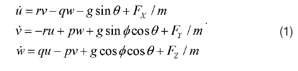
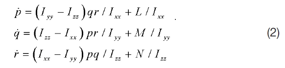
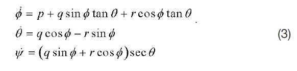
Considering the size of multi-rotor UAVs relative to their surroundings, they are assumed to be rigid objects. The multirotor UAV is free to rotate and translate in three-dimensional(3D) space, and the rigid body dynamics are derived by Newton’s laws (Stevens and Lewis, 2003). For multi-rotor UAVs, the 6-degree of freedom rigid-body equations of motion are expressed as the differential equations describing the translational motion, rotational motion, and kinematics,as given below.
In the above, (
Force equations
Moment equations
Kinematic equations
gravity with respect to the body-fixed frame. (
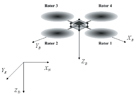
2.2 Configurations of quad-rotor UAV
In this section, the configuration of the quad-rotor is introduced, as shown in Fig. 2.
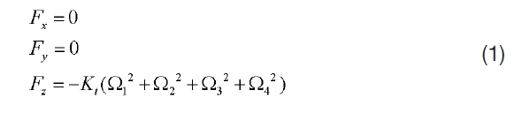
The quad-rotor UAV contains four rotors, of which two rotors rotate in the same direction, whereas the other two rotate in the opposite direction. As shown in Fig. 2,the quadrotor UAV gains its total thrust by the combination of the four rotors. The rotor numbers are shown in Fig.2 : rotor 1 is the head and rotor 3 is the tail of the system. In addition, rotors 1 and 3 rotate in the clockwise direction, whereas rotors 2 and 4 rotate in the counterclockwise direction. There are several advantages in having such a configuration. First of all, this
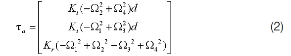
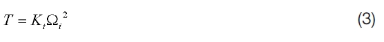
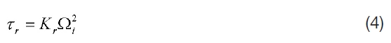
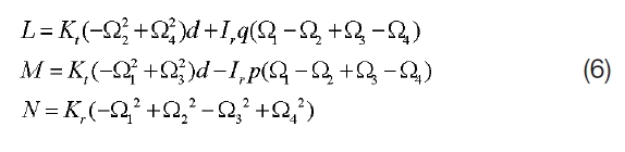
system does not require a swash plate, which is necessary to change attitude in a conventional helicopter, since it changes its attitude by varying the angular speeds of the rotors. Also, it overcomes the reactive torque of the system, since it contains an even number of rotors. This means that by rotating rotors 1 and 3 in one direction and rotors 2 and 4 in the other direction, the reactive torque of the system is cancelled out automatically. The forces and moments generated in this system are listed in Eqs. (1) and (2).
where
The gyroscopic torques due to the combination of the rotation of the airframe and the four rotors are given by:
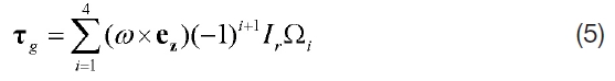
where ez=[0, 0, 1]
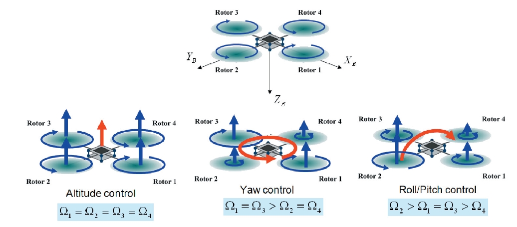
2.3 Control strategies of multi-rotor UAVs
Control strategies of multi-rotor UAVs include attitude control and position control. In order to generate the position control, attitude control should be done first. Therefore, this section mostly deals with the attitude control strategies of the quad-rotor UAV. Figure 3 shows the attitude control strategies of the quad-rotor UAV.
As Fig. 3 shows, the attitude control of the quad-rotor is performed by varying the angular velocities of the rotors. For example, altitude control is done by increasing the angular speeds of the four rotors simultaneously, and the yaw and pitch/roll controls are done by varying the angular speeds of one or two rotors as shown in Fig. 3 Due to the use of this mechanism, this system does not require a swash plate for attitude changes.
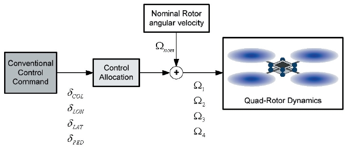
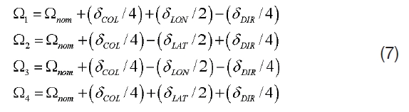
2.4 Control allocation of multi-rotor UAVs
Since multi-rotor UAVs have multiple rotors and only use the rotors’ angular speeds for the control of the UAV, a proper control allocation method is necessary. Typical helicopter commands are also used in these multi-rotor UAVs: they areδ
3. Vision Based Collision Avoidance
In this section, the vision-based collision avoidance technique is introduced. For the multi-rotor UAVs to maneuver in a safe and stable manner, a proper algorithm is required to provide an effective obstacle avoidance technique. One of the most widely known collision avoidance techniques is the optical flow method. The optical flow is the relative movements of the pixels from one frame to the next and is represented as a velocity vector. As the UAV operates in places such as offices, disaster sites, steep terrains, etc., it inevitably encounters numerous obstacles. In order to avoid such obstacles, well calculated optical flow information from the camera is necessary. The next section deals with the optical flow estimation based on the Lucas-Kanade (LK)optical flow algorithm.
The Lucas-Kanade algorithm is one of the most famous optical flow methods and (was originally developed?) by B. Lucas and T. Kanade in 1981. The LK algorithm is based on the following three assumptions (Bradski and Kaehler,2008; Sonka et al., 2008). First, the LK algorithm assumes the constant brightness, which means that the brightness of every pixel in a frame maintains its brightness all the way through. Secondly, the LK algorithm has temporal persistence or “small movement” properties, which means that the movement of the object over time is not significant.Finally, the LK algorithm assumes spatial coherence,meaning that spatially adjacent pixels tend to belong to the same object and also tend to have identical movements. With the above three assumptions, a proper estimation method for the optical flow can be obtained.
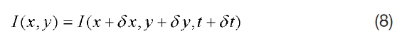
In order to calculate the optical flow, we assume that the intensity I of a frame is constant throughout the time from t to t+δt. Then, we may obtain the following constraint equation(Muratet et al., 2004, 2005).
By applying the Taylor series to Eq. (8), we can obtain Eq.(9).
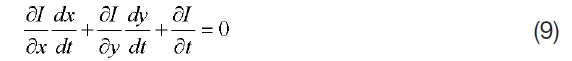
where
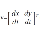
denotes the optical flow of a pixel I(x,y) in an image, and
and

represent the spatial derivatives and brightness intensity variance over time, respectively. We may rewrite Eq. (9) in different ways,such as Eqs. (10) and (11).


where u=[u v]T and I=[Ix Iy]T in Eq. (10).
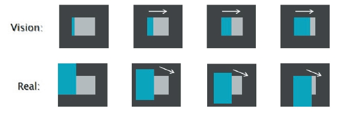
Equation (11) is related to one pixel of a frame, which means one equation with two unknowns. Thus, the measurement information from a pixel cannot give a unique solution with respect to 2D movements: it can only obtain the solution in the normal directional component. This problem arises from the aperture problem, which arises when estimating a movement from a small hole or window. Let us assume that we are observing the movement of a wide object with the same color in the eastward direction through a small hole or window. We cannot tell whether it is moving in the eastward direction or north-east direction by observing only the movement of its edges; this is the aperture problem.
To overcome this problem, recalling the third assumption of the LK method, we are able to obtain the movement of the
center pixel, which can be derived from the pixels around it.This statement can be expressed in the form of an equation,as follows :
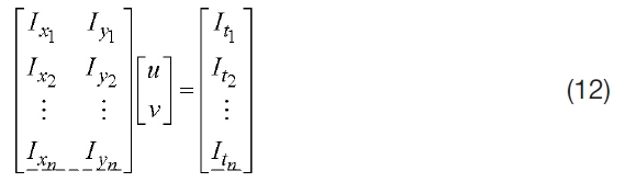
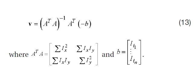
Equation (12) represents an over-constrained system,which could give a solution from a single edge viewed from a window. In order to solve Eq. (12), the method of least squares is used, and the result of the optical flow is obtained as shown in Eq. (13).
3.3 Application to multi-rotor UAV
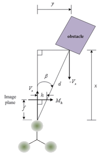
In order to apply the optical flow method to the multirotor UAV, the geometry of the relationship between the UAV and obstacle in Fig. 6 is effectively used. As the coordinate is defined as shown in Fig. 6, it is assumed to be a 2D optical flow problem (Park et al., 2008; Souhila and Karim, 2007).
In Fig. 6,
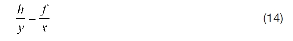
Rearranging and differentiating Eq. (14) with respect to the time, we obtain
By using the facts y=?, ?=-Vx and ?=Mh, one can obtain(
By replacing x by d cos
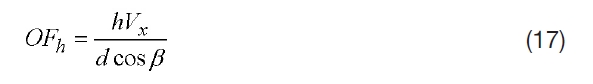
From Eq. (17), it can be seen that, surprisingly, as the relative distance d decreases, the optical flow value becomes larger and vice versa. When the optical flow value increases,meaning that the obstacle comes close to it, the UAV has to perform an avoidance maneuver. This leads to a strategy called the ‘balance strategy,’ which tends to maintain the optical flows of the right and left sides of the vehicle at equal distances. When the UAV calculates the optical flow data using Eq. (17), the balance strategy suggests that the UAV will turn to the right if the optical flow from the left side is greater than the optical flow from the right side of the screen and vice versa. For example, if there is an obstacle in the forward-right direction of the UAV, as shown in Fig. 6, the optical flow value of the right side increases and the UAV turns to the left. This behavior is derived as an equation, as shown in Eq. (18).
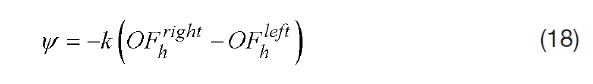
where ψ is the input value of the yaw angle of the multirotor UAV, OFh right is the optical flow value obtained from the right side, OFh left is the optical flow value obtained from the left side, and k is the proportional constant. As Eq.(18) suggests, the multi-rotor UAV performs the collision avoidance maneuver with the input value of the yaw angle,which is related to the δped command. The next section describes the simulation results of the multi-rotor maneuver in virtual 3D space.
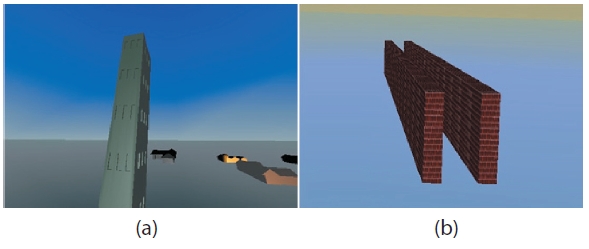
In order to test the collision avoidance algorithm, a quadrotor model is used to navigate in various virtual 3D spaces,as mentioned above. The virtual 3D spaces are designed as urban environments that UAVs could easily encounter in real life. In this simulation, the 3D virtual spaces selected are buildings and corridors and are shown in Fig. 7.
The virtual 3D spaces are designed with the virtual reality program in MATLAB. The quad-rotor used in this simulation weighs 1.1 kg and the distance from the center of mass to each rotor axis and the radius of the spinning rotors are set to 0.24 meters and 0.01025 meters, respectively.
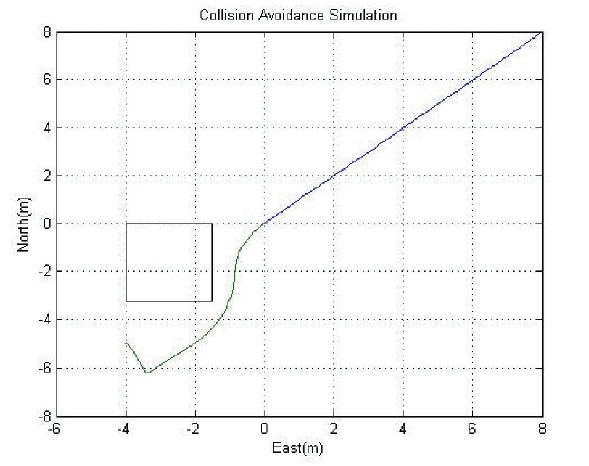
The image processing frequency was set to 10 Hz. As shown in Fig. 7,scenario (a) is for the quad-rotor UAV to fly to the designated arrival point while avoiding colliding into the tall building, which is right on the UAV’s path to the destination.The initial position of the UAV was set to (8 m, 8 m) and the final position was set to (-5 m, 4 m), as represented in Fig..8 The initial heading angle of the quad-rotor was set to 225 degrees and the vehicle’s initial speed was set to 2 m/s. The simulation result is shown in Fig. 8.
As shown in Fig. 8,the square on the graph represents the position of the building and the trajectory of the UAV, shown
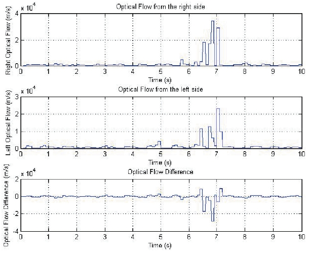
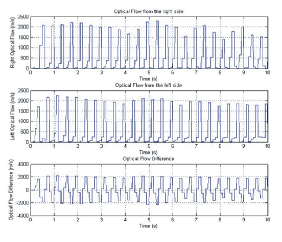
as a mixture of blue and green lines, indicates that the quadrotor initiates its avoidance maneuver at around the (0 m,0 m) point and travels around the building. Figure 9 shows the optical flow values obtained from the right, left, and difference between the right and left. As shown in Fig. 9,as the UAV approaches the left side of the building, the optical flow value of the right side of the UAV is greater than that of the left side, which leads to the UAV’s changing its heading toward the left.
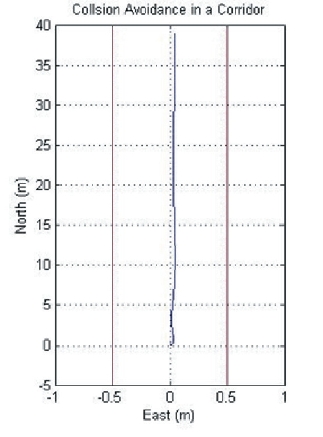
Another simulation was conducted, in which the UAV cruises along a corridor, as shown in Fig.7 b. In this case,the UAV has to fly between the two walls with its lateral position located in the middle of the corridor. The distance between the two walls is set to 1 meter. The initial velocity of the UAV was 0 m/s, meaning that it started from the hovering position. However, the initial pitching angle of -5
degrees gave the system some forward movement. Figure 10 shows the trajectory of the UAV. Figure 10 indicates that the UAV navigates safely in the middle of the corridor without crashing into the wall.
Figure 11 shows the right and left optical flow values and the differences between them. By observing the behaviors of the UAV in the above two simulations, it can be seen that the 2D collision avoidance of the multi-rotor UAV by optical flow is successfully accomplished. It must be noted that, in this simulation, the relative distances between the obstacles and UAVs are known factors, since this simulation assumes that the vehicle has the information about the location of the obstacle and its own states. However, to implement this in a real life experiment, the vehicle should contain a global positioning system (GPS) and a relative distance calculation algorithm based on a vision system. One suggested strategy to calculate the relative distance is to apply stereo vision technology, which uses two cameras to estimate the distance from the camera to the obstacle.
In this paper, the collision avoidance of multi-rotor UAVs by optical flow is introduced. First, as one type of multi-rotor UAV, the dynamics and control strategies for a quad-rotor UAV were introduced, as well as its control allocations. In order for a UAV to navigate safely in urban areas for various missions, an autonomous collision avoidance technique should be implemented in the system. As one of the collision avoidance techniques, the optical flow method derived by LK was introduced. By using the vision information obtained from the camera on the UAV, the optical flow data can be calculated by applying the LK method to every frame. After obtaining these optical flow results, one can apply them to the geometry between the UAV and an obstacle ahead.Finally, by using a balance strategy, the UAV is capable of steering away from dangerous obstacles autonomously.This theory is applied to a virtual 3D environment in order conduct simulations. The simulation results indicate that the quad-rotor UAV successfully achieves 2D autonomous obstacle avoidance. In the future, based on the results obtained from the simulation, we will extend the scope of this study to the real world implementation of obstacle avoidance by performing a number of experiments on an actual quad-rotor UAV. In order to use the proposed method in a real life experiment, GPS and stereo visions are required to be applied in order to acquire the positions of both the vehicle and obstacles.