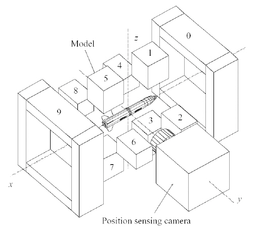
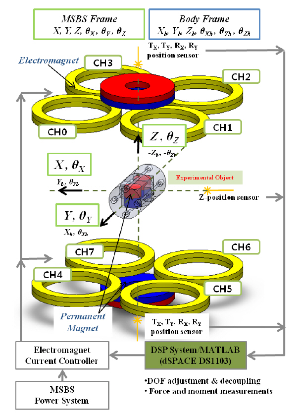
Wind tunnel tests are often used observe the air flow around an aerodynamic body as well as measure the aerodynamic forces acting on an aerodynamic body.Oftentimes, mechanical supports are employed in order to fix the aerodynamic body at the center of the test section.However, these mechanical supports cause disturbances to the air flow around the aerodynamic body, decreasing the accuracy of the experimental results. Magnetic suspension and balance systems (MSBSs) provide ideal solutions for these disturbance problems. An MSBS has the ability to levitate the magnetized model at the center of the test section of a wind tunnel without any mechanical support, such as sting or strut, by using magnetic forces and moments(Figs. 1 and 2). Thus, an aerodynamic model, which is partially or fully composed of ferromagnetic material, can be suspended in the test section by an MSBS. One point to note is that the remaining portions of the aerodynamic model not composed of ferromagnetic materials must be made of a rigid, electrically non-conducting material in order to avoid side effects caused by electromagnetic fields. Meanwhile,an MSBS can easily change the position and attitude of the model as well as measure the external forces and moments simultaneously acting on the model while refraining from physical contact. Thus, an MSBS eliminates support interferences during wind tunnel tests (Covert, 1988).
The basic idea of MSBSs was originally proposed by Holmes
(1937). He suggested that magnetic forces can be used to reduce frictional forces acting on bearings. Subsequently,an MSBS was successfully developed for wind tunnel tests by Laurenceau et al. (1957). As a result, MSBSs were mostly utilized to eliminate support interferences during wind tunnel tests. The advantage of eliminating support interferences is most helpful during wind tunnel tests under super sonic conditions. Using an MSBS, Owen et al. (2007)measured the lift and drag coefficients of a cone under a supersonic regime, thus eliminating shock interferences caused by stings or supports in other systems. Sawada et al.(2004) used the MSBS installed on the JAXA subsonic wind tunnel in order to measure the drag coefficients of a sphere.Higuchi et al. (2006, 2008) observed the air flow around several cylinders with particle image velocimetry during wind tunnel tests with the same MSBS. Additionally, Higuchi et al. (2006, 2008) also measured drag coefficients and the base pressure of these cylinders.
Regardless of the advancements made in regards to MSBSs,further development of an improved MSBS is still needed,requiring greater effort and increasing costs. In particular, the size of an electric power supply system and cooling system for the electromagnet is substantially increasing as demands of specific MSBS functions increase, thus increasing the costs of MSBS research and development efforts (Covert, 1988).Consequently, developing an MSBS without performance prediction carries more risks. Performance should then be predicted during the design process. In this study, magnetic fields generated by electromagnets and permanent magnets of an MSBS were modeled under certain assumptions. The calculated results were compared to experimental results as a means of verifying the assumptions. Relationships between state/control variables and magnetic forces/moments were also obtained in state space form so that the 6-degree of freedom (DOF) control simulation was performed with the system matrix of the MSBS. 6 independent proportionaldifferential controllers were used for each DOF in the simulation. Finally, 6-DOF control simulator was developed and the performance of the MSBS was successfully predicted with step-response simulation and an external force measurement simulation.
The equation describing the motion of a rigid body in the body fixed system can be expressed as follows:
where
represent the mass of the body,the linear and angular velocities, the linear momentum and the angular momentum, respectively.
are the external forces and external moments acting on the body. For an aerodynamic model located in the MSBS with no air flow,the gravitational force and the magnetic forces and moments are the only external forces and moments that exist. These forces can be rewritten as
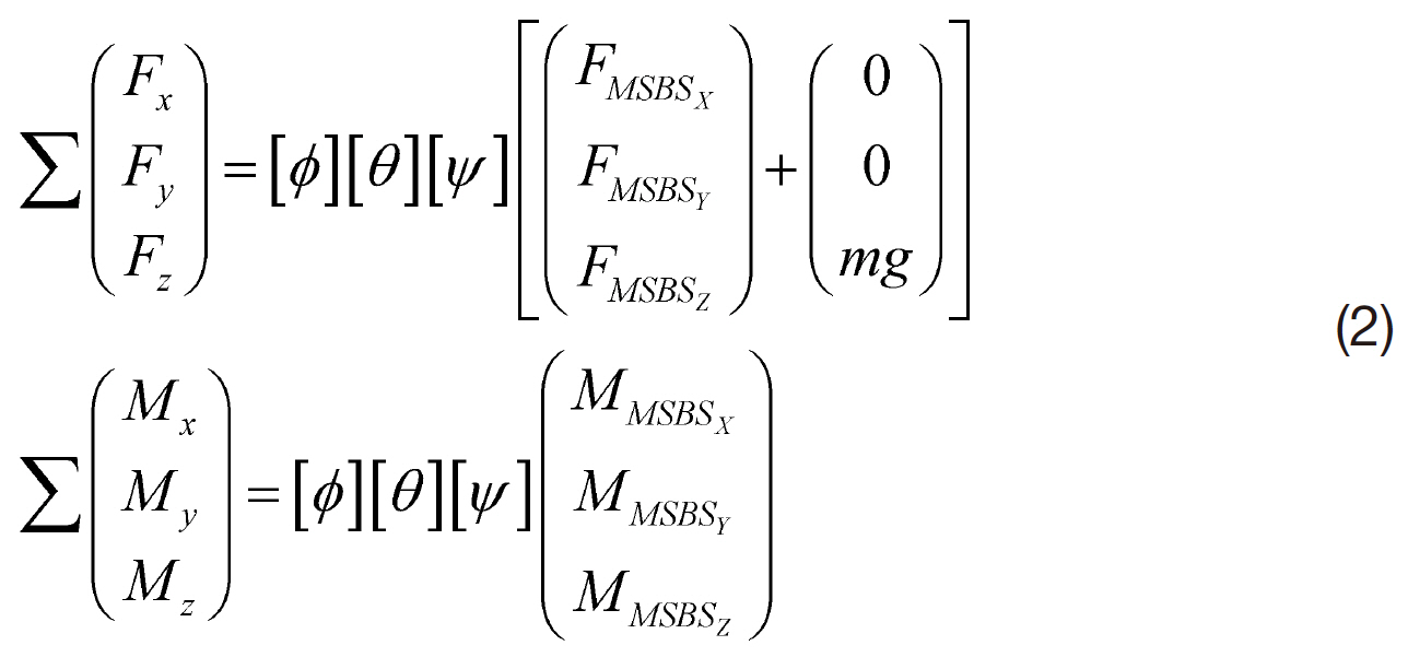
where FMSBSx, FMSBSy, FMSBSz denote the X, Y and Z components of the magnetic force, and similarly FMSBSx, FMSBSy, FMSBSz are the X, Y and Z components of the magnetic moment,respectively. [φ][θ][ψ] is the transformation matrix that converts the force and moment expressions from the MSBS fixed frame to the body fixed frame. Therefore, if the magnetic forces and moments generated by the MSBS were appropriately obtained, the equation of motion of the aerodynamic model can be completely defined and can be expressed in state space form by applying the small disturbance theory.
The magnetic force exerted on the point charge

is
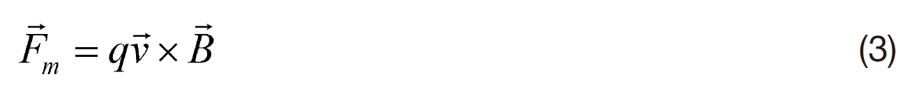
if a magnetic field

exists. The magnetic field can be generated by another moving charge q1 as follows:
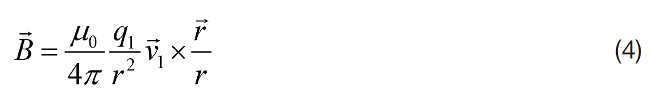
where

is the position vector from q1 to q,

is the velocity vector of q1

is known as
With Eq. (3), the magnetic force acting on a conducting wire

generated by magnetic field
can be obtained. If a conducting wire
with cross section A is placed inside the magnetic field
and N point charges of quantity q move in the conducting wire with the velocity
then the force acting on the conducting wire is
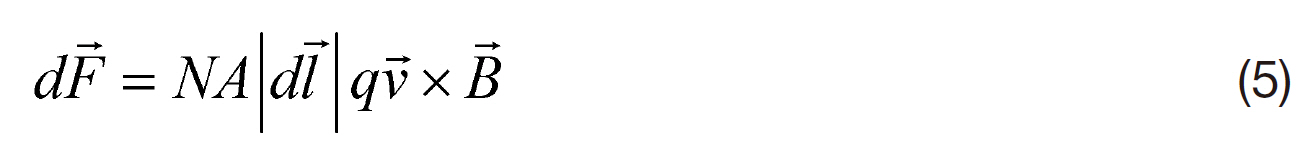
Since
are parallel to each other, Eq. (5) can be reduced to
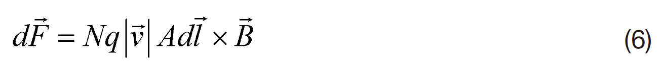

in Eq. (6) means the electric current I, and

can be simply expressed as

In the same context, when the electric current I1 flows through a conducting wire

located at

from the origin and the electric current I2 flows through a conducting wire
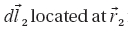
from the origin, the magnetic force acting on the conducting wire

generated by magnetic field from a conducting wire
can be written as
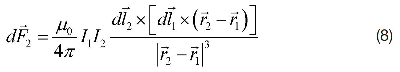
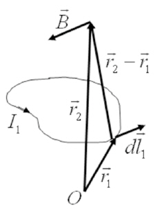
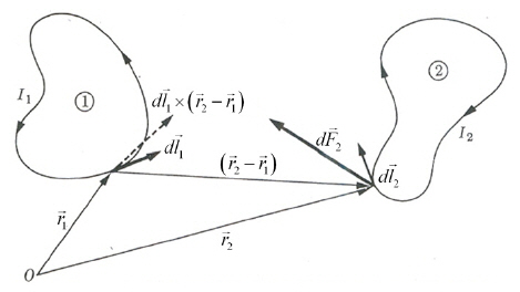
When these conducting wires

form closed curves, as shown in Fig. 3,the magnetic force acting on closed curve No. 2 can be obtained by integrating Eq. (8) as follows:
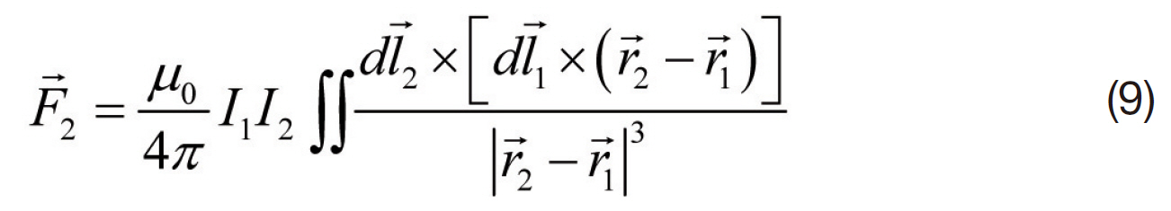
Meanwhile, the magnetic field
generated by an arbitrary current circuit through which electric current I1 flows (Fig. 4)can be written as follows.
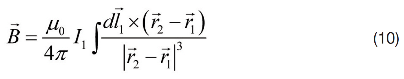
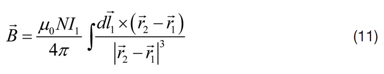
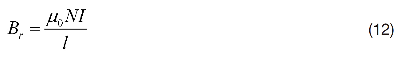
Thus the magnetic field generated by an electromagnet can be calculated by Eq. (11) if it is modeled as a circular coil(Christy et al., 1993).
where
The MSBS studied in this paper comprised a 33 cm × 40 cm test section. The system was composed of two large permanent magnets and eight electromagnets, as shown in Fig. 5. The outer and inner diameters of the electromagnets were 180 mm and 140 mm, respectively. The thickness of the magnet was 20 mm, and the number of turns was 255. The large permanent magnets were made of samarium-cobalt,of which its remanence was 1.066 T. The large permanent magnets possessed dimensions of 150 mm as the outer diameter, 50 mm as the inner diameter, and 25 mm in thickness.
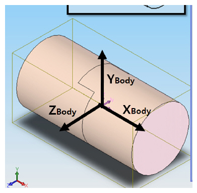
This study employed a cylinder type object, as shown in Fig. 6, as the aerodynamic model. The mass of the model was measured by an electronic scale and the moment of inertia of the model was obtained from a 3D CAD program.The values of the mass and the moment of inertia of the aerodynamic model are shown in Table 1. The aerodynamic model contained several small permanent magnets in
order to react to the magnetic field generated by the MSBS.The small permanent magnets were made of neodymium with a remanence of 1.39 T. The permanent magnets were cylindrical in shape, possessing dimensions of 35mm in diameter and 40 mm in thickness.
[Table 1.] Mass and moment of inertia of the cylinder model obtainedfrom CAD program

Mass and moment of inertia of the cylinder model obtainedfrom CAD program
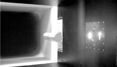
The MSBS had the ability to countervail the weight of the aerodynamic model with the magnetic forces generated by the two large permanent magnets. It controlled the position and attitude of the model through active control using eight electromagnets. The changes in position and attitude of the model were continuously detected by several laser sensors, and a microprocessor provided the control signals in real-time to generate appropriate input currents for each electromagnet.
3.2 Magnetic field
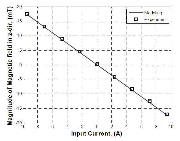
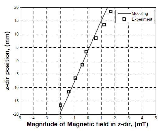
Eq. (11) was used to calculate the magnetic fields generated by the electromagnet. The electromagnet was modeled as a circular coil with 255 turns and an average diameter of 160 mm. The calculated magnetic fields were compared to the experimental results for various input currents. As shown in Fig. 7, the magnetic field in the z-direction parallel to the axial direction of the electromagnet measured at the 20 mm above the center of the electromagnet (X = 0 mm, Y = 0 mm, Z= 20 mm) and it is consistent with the simulated result.
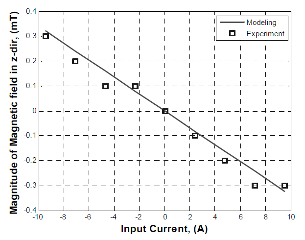
Figure 8 shows the magnetic field in a different position(X = -95 mm, Y = -95 mm, Z = 93.5 mm). Slight differences exist between the simul ated and measured magnetic fields illustrated in Fig.8. This discrepancy was caused by the limit of the sensor resolution. The experimental results, measured by a Gauss meter with a resolution of 0.1 mT, were bounded within 0.1 mT. Through the comparisons, the conclusion follows that electromagnets can be modeled as circular
[Table 2.] The major parameters for modeling the permanent magnets as circular coils
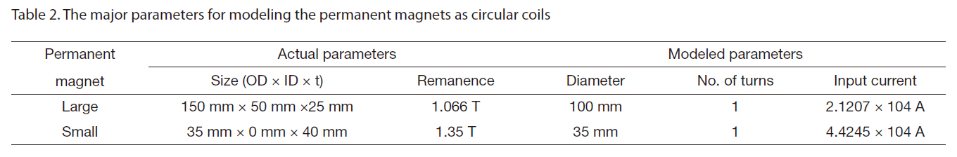
The major parameters for modeling the permanent magnets as circular coils
coils.
The large permanent magnets for the MSBS and the small permanent magnets used in the aerodynamic model were modeled as coils with some assumptions on dimensions arranged in Table 2. The large permanent magnet was modeled as a coil and the diameter of the modeled coil was the mean value of the inner and outer diameters of the large permanent magnet. The small permanent magnet was modeled as a coil which possessed same diameter with the small permanent magnet. The number of turns was assumed as one, and each magnitude of the input current for each modeled coil was calculated using Eq. (12) with the known thickness, the number of turns and the remanence of each permanent magnet (Christy et al., 1993).
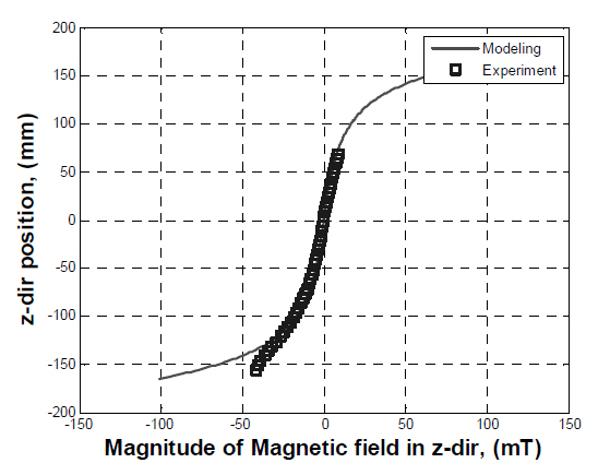
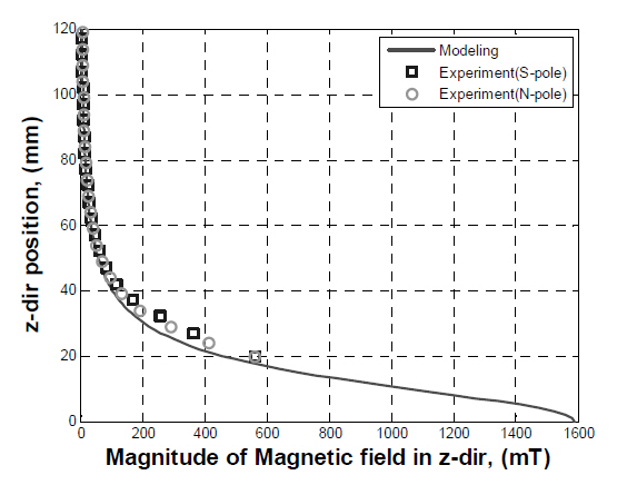
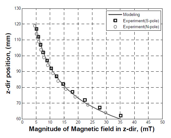
The magnetic fields generated by the two large permanent magnets in the MSBS were modeled as a system with two coils at the top and bottom. The calculation was performed along the axis of the permanent magnets. The results from the calculation were compared to the experimental results.Figure 9 shows the magnetic field distribution for the entire domain, and Fig. 10 represents an enlargement of the same results for the operating domain. The calculated and measured results are the same on the operating range determined to be near the middle of the two permanent magnets, indicating that the large permanent magnets can be modeled as coils.It was observed that the difference between the measured and simulated results increases as the z-directional position approaches the permanent magnet. This difference originates from the assumption that permanent magnets may be modeled as coils. The magnetic fields generated by the small permanent magnet were calculated in the same manner as the large permanent magnets, represented in Figs. 11 and 12.The calculated magnetic fields correspond to the measured magnetic fields in the operating domain, indicating that the small permanent magnet can be also modeled as a coil.
Based on the results obtained from the aforementioned
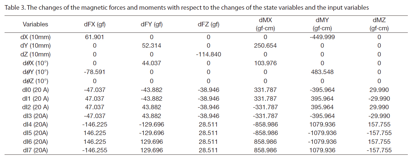
experiments, it is believed that the magnetic fields generated by the electromagnets and the permanent magnets can be calculated by modeling these magnets as coils, allowing researchers to obtain the magnetic forces and moments existing between these magnets using Eq. (9). The two large permanent magnets of the MSBS countervail the weight of the aerodynamic model in the MSBS. Calculations show that the weight equilibrium position of the model is directly below 40 mm in z-direction from the center of the MSBS. After calculating the magnetic forces and moments for various ranges of state variables and input variables, it was observed that the relationships between the magnetic forces/moments and the state/input variables appear linear around the weight equilibrium position. Thus the force/moment derivatives with respect to the state/input variables could be extracted as shown in Table 3, while relatively small amounts of change were neglected. These derivatives were
used to obtain the equation of motion of the aerodynamic model in state space form so that the simulation of motion of the model can be performed efficiently.
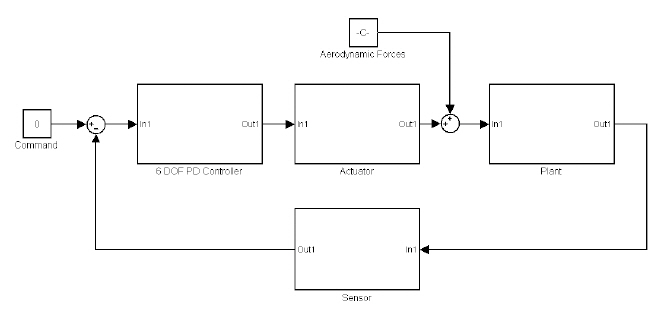
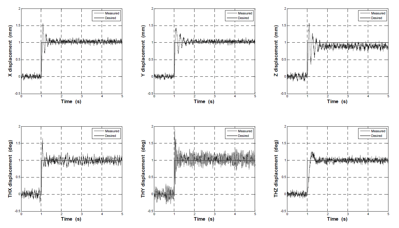
The equation of motion of the aerodynamic model in the MSBS, which was obtained in state space form, was imported into MATLAB Simulink to simulate 6-DOF control, as shown in Fig. 13. Limiting factors, such as the operating range and the actuator delay of electromagnets, were modeled. The sensor noise was also modeled in the simulation block.Six independent proportional-differential controllers were employed to control each DOF, and the control gains were obtained in accordance to classical control theory.In the end, the 6-DOF control simulator of the MSBS was developed to allow performance predictability of the MSBS. As shown in Fig. 14, a step response simulation was
performed and the root mean square errors (RMSEs) for each DOF were calculated in order to quantitatively evaluate the performance. The calculated RMSEs for X, Y, Z, θX, θY and θZ were 0.0851 mm, 0.0842 mm, 0.1146 mm, 0.0911°,0.1411° and 0.0975° respectively. These results ensure that the MSBS possesses sufficient performance needed to fix the aerodynamic model around the weight equilibrium position inside of the MSBS.
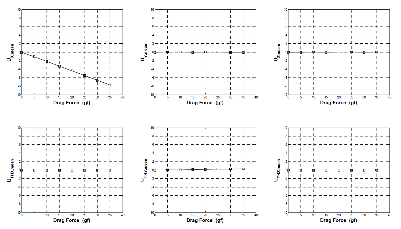
3.5 External force measurement
An MSBS not only acts as contactless actuator but also contactless balance, facilitating the measurement of external forces acting on an aerodynamic body within the system while forcing the position and the attitude of the body to follow the demanded values. When wind tunnel tests using an MSBS are performed, the equation of motion of the aerodynamic body can be expressed as follows.
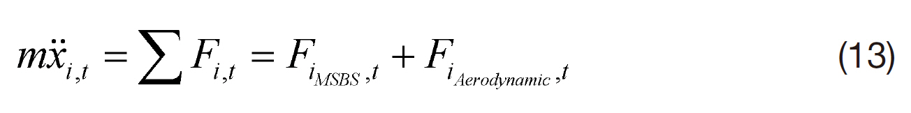
where

The changes of the magnetic forces and moments with respect to the changes of the state variables and the input variables
of the equation, such as
This study developed a 6-DOF control simulator for an MSBS. The MSBS contained eight electromagnets and two permanent magnets as well as an aerodynamic model. The aerodynamic model remained at the weight equilibrium position within the MSBS. In addition, the model comprised
of several permanent magnets to handle magnetic forces and moments generated by the MSBS. The two permanent magnets countervail the weight of the model and the eight electromagnets control the 6-DOF of the model.These magnets were modeled as coils in order to calculate the magnetic forces and moments. Subsequently, the eight electromagnets control the 6-DOF of the model.These magnets were modeled as coils in order to calculate the magnetic forces and moments. Subsequently, the relationships between the magnetic forces/moments and the state/input variables were obtained in order to extract the force and moment derivatives. The equation of motion of the model was obtained in state space form and the 6-DOF control simulation was performed using this equation. The simulator developed in this study successfully predicted the performance of the MSBS. The step response simulation result indicated that the MSBS can hold the aerodynamic model around a specific position. Furthermore, wind tunnel test simulations confirmed that the MSBS can measure the external forces, such as drag forces, acting on the aerodynamic body during the tests.