There are various difficult situations where an individual cannot do his job properly, such as working in steep terrains,disaster sites, military operational areas, or small indoor facilities. Since working in such areas requires massive equipment for conducting missions, proper solutions are needed for those situations. In order to facilitate work in such difficult situations, unmanned aerial vehicles (UAVs)have been regarded as the proper solution, and many studies relating to this topic are still underway. There are several requirements for UAVs that are used in such areas. First,the UAV should be small-sized in order to guarantee its free motion under any circumstances. Second, the UAV requires rapid motion in every possible direction so that it can avoid a sudden collision. Finally, the UAV needs to be capable of vertical takeoff and landing, and also achieve sudden directional turns. To satisfy all the above requirements,a multi-rotor thrust UAV is considered to be the best solution for this scenario. Multi-rotor UAVs are of various kinds including bi-rotor, tri-rotor, quad-rotor, and also the conventional helicopter type (Guenard et al., 2005; Tayebi and McGilvray, 2004). Of these types of design, the tri-rotor,which has three axes of rotation that form a triangular shape,is the main concern of this paper.

The tri-rotor UAV has the problem of having a yawing moment that is induced by the reaction torque from the unpaired rotor. In order to solve this problem, several designs of tri-rotor UAV have been developed with their own solutions. The first type is called ‘single tri-rotor,’ and was studied by University Technology of Compiegne (Salazar-Cruz et al., 2008). The main idea of this type is that a servo motor is installed on one of the rotor axes, which gets tilted by some angle to nullify the yawing moment (Escareo et al.,2008). The main advantage of this design is better movement,especially for a quicker turn, by the tilting of one of the rotor axes (Salazar-Cruz and Lozano, 2005). The other type of trirotor UAV is called ‘coaxial tri-rotor’; Draganflyer X6 from Draganfly Innovation Inc. (Saskatoon, Canada) could be considered as being of this type. It has two rotors installed on each rotor axis, and thus, six rotors in total. By the presence of two counter-rotating rotors on each axis, the reaction torque naturally has been nullified. This type of tri-rotor guarantees better stability than single tri-rotor UAVs.

In this paper, a small-sized tri-rotor UAV with vertical takeoff and landing abilities has been considered and described. In order to apply the tri-rotor concept to real-world flying UAVs, hardware testing is necessary for both types of tri-rotor. Before experimental testing, numerical simulations of a nonlinear system of UAVs should be conducted. Thus,control strategies are proposed for both types of tri-rotor,and nonlinear simulations of the altitude, Euler angle, and angular velocity responses have been conducted by using a classical proportional-integral-derivative (PID) controller.This paper is organized as follows. In Section 2, the rigid body equations of motion of tri-rotor UAVs are explained. Then,the control strategies of both single and coaxial tri-rotors are introduced as well as their force and moment equations.Control system designs are introduced in Section 4 for both tri-rotors. Finally, nonlinear simulation results are presented for altitude and attitude control.

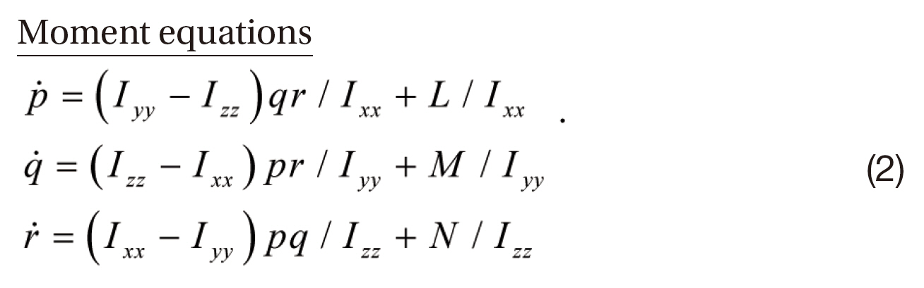
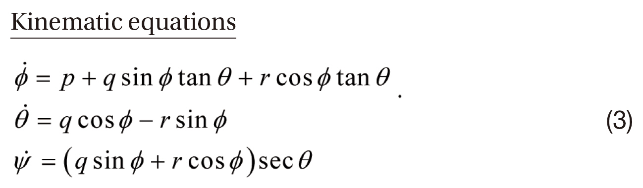
Considering the size of tri-rotor UAVs relative to the surroundings, tri-rotor UAVs are assumed to be rigid objects.The 6-degree of freedom (DOF) nonlinear equations of motion that are developed for conventional UAVs are also used for tri-rotor UAVs. The tri-rotor UAV is free to rotate and translate in three-dimensional space, and the rigid body dynamics are derived by Newton’s laws (Mettler, 2003;Stevens and Lewis, 1992). For tri-rotor UAVs, the 6-DOF rigidbody equations of motion are expressed as the differential equations describing the translational motion, rotational motion, and kinematics as given below.

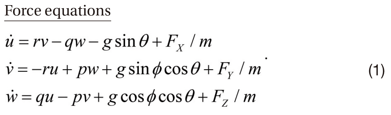
In the above, (F_x, F_y, F_z) are the external forces, and (L,M, N) are the external moments acting on the center of gravity with respect to the body-fixed frame. (u, v, w) are the translational velocities, (p, q, r) are the rotational velocities,and (φ, θ, ψ) are the rotational angles. I_xx, I_yy, and I_zz are the rotational inertias of the tri-rotor UAV.

A single tri-rotor has three rotors, and one of the rotors,the tail-rotor to be specific, is tilted to nullify the effect of the reaction torque of the system. A single tri-rotor has the advantage of the generation of rapid motion from its tilt rotor, which could also be a challenge for this system since it requires a very accurate value of the tilting angle for stabilization of the system.

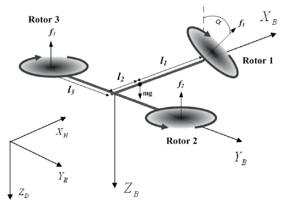
Figure 1 shows the configuration of a single tri-rotor UAV with the reference and body frames.

As shown in Fig. 1, the distances, l₁, l₂, and l₃, are defined,and the distances from the center of gravity to each rotor are identical. Two front rotors, rotors 2 and 3, rotate in other directions, and the tilting rotor, rotor 1, rotates in the same direction as rotor 3. Therefore, without tilting rotor 1, the whole system tends to have a yawing moment in the counterclockwise direction, and this is the reason for having a servo motor on the rotor-1 axis for tilting purposes. As rotor 1 tilts as shown in Fig. 1, it creates a moment that cancels the

yawing moment of the system. A very accurate calculation of the tilting angle, α, is essential for this system since it has the role of three degrees of freedom motion control as well as hovering control. The force and moment equations of the single tri-rotor UAV are derived with respect to Figure 1,and are expressed in Eqs. (4) and (5).

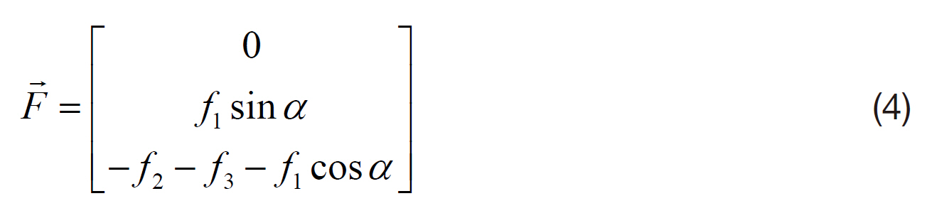
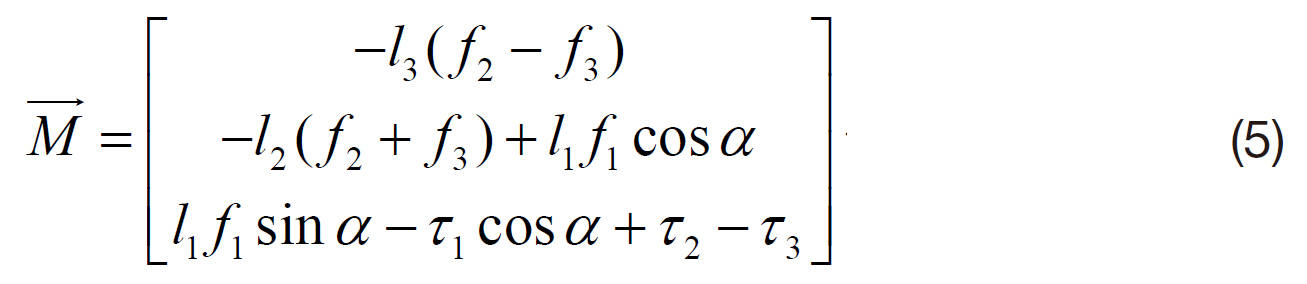
In the bove, a is the tilt angle of rotor 1, as shown in Fig. 1. f₁, f₂, and f₃ are the rotor forces, and τ₁, τ₂, and τ₃are the rotor torques; these are defined in Eq. (6). K_t and K_τ are the thrust and torque coefficients, and Ω is the angular velocity of the rotor.

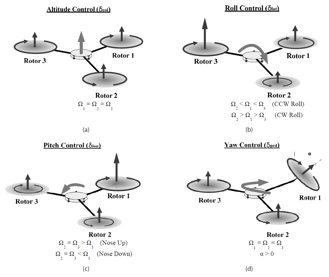
As mentioned above, the tilting angle, α, plays an important role in single tri-rotor control. The tri-rotor’s motion control can be decomposed into altitude, roll, pitch,and yaw control. The control strategies of single tri-rotors are shown in Fig. 2. Fig. 2(a) shows the altitude control and that increasing the speed of each rotor will increase the altitude,and vice versa. Fig. 2(b) shows the roll control; the approach towards roll control is that given the same rotor-1 speed,varying the rotor speeds of the two front rotors will generate roll control. Figure 2(c) shows the pitch control; given the same angular velocities for the front two rotors, varying the rotor speed of rotor 1 will generate pitch control. Regarding the yaw control, by using the natural yawing moment from the reaction torque and also from the tilt angle, α, yaw control can be successfully generated. The tilt angle, α, is very useful when encountering a sudden danger of collision because by tilting the rotor, sudden turning control would be possible.

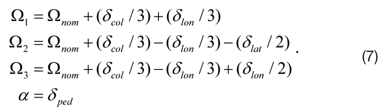
For the successful and stable control of tri-rotor UAVs,accurate control allocation is essential. The tri-rotor

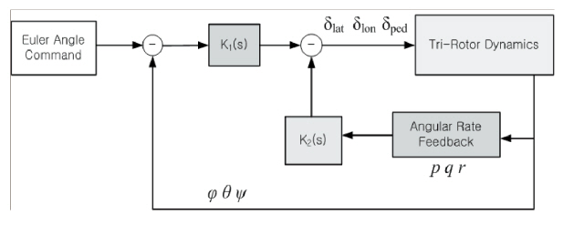
will follow a control command similar to conventional helicopter control commands, which are collective, lateral,longitudinal, and yaw or pedal (Padfield, 2007). They are expressed as δ_col' δ_lat' δ_lon' and δ_ped.The single tri-rotor UAV will be controlled by the angular velocities of the three rotors and the tilt angle of rotor 1. Figure 3 and Eq. (7) show the control allocation of a single tri-rotor. Figure 4 shows a block diagram for the attitude hold autopilot of the single tri-rotor UAV. The attitude hold autopilot tracks the pitch, roll, and yaw angles, and holds them. As shown in Fig. 4, the attitude hold autopilot consists of a double loop, wherein the inner loop represents angular-rate feedback, and the outer-loop represents attitude feedback (Castillo et al., 2004).

In Fig. 4, K₁ and K₂ are the gain values of the Euler angle attitude and angular rate, respectively.

A coaxial tri-rotor UAV has two rotors installed on each axis of rotation; therefore, the system has six rotors in total.Through counter-rotating rotors on each axis, it is possible to nullify the yawing moment on each axis as well as on the whole system. The advantage of this system is better stability, but more power is required for six rotors?which is a disadvantage of the system.

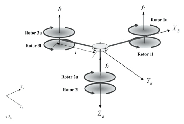
The coaxial tri-rotor’s configuration with the body and reference frames is shown in Fig. 5.

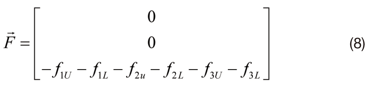
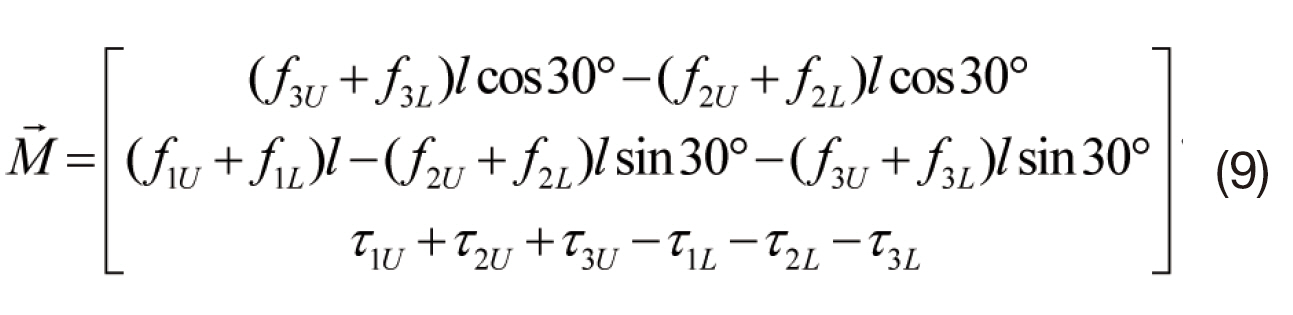
As the figure shows, each axis of rotation contains upper and lower rotors. All upper rotors rotate in the clockwise direction, and all lower rotors rotate in the counter-clockwise direction. Because of this behavior, the coaxial tri-rotor UAV does not need an extra device, such as the servo motor used for single tri-rotors, in order to nullify the yawing moment of the system. The distances from the center of gravity to each rotor are the same and defined as l. The force and moment equations were derived with respect to Fig. 5, and are expressed in Eqs. (8) and (9). Again, as mentioned above,f_1' f_2'and 2₃ are rotor forces and τ₁, τ₂, and τ₃ are rotor torques,and the subscripts, U and L, under rotor torques refer to‘Upper’ and ‘Lower,’ respectively.

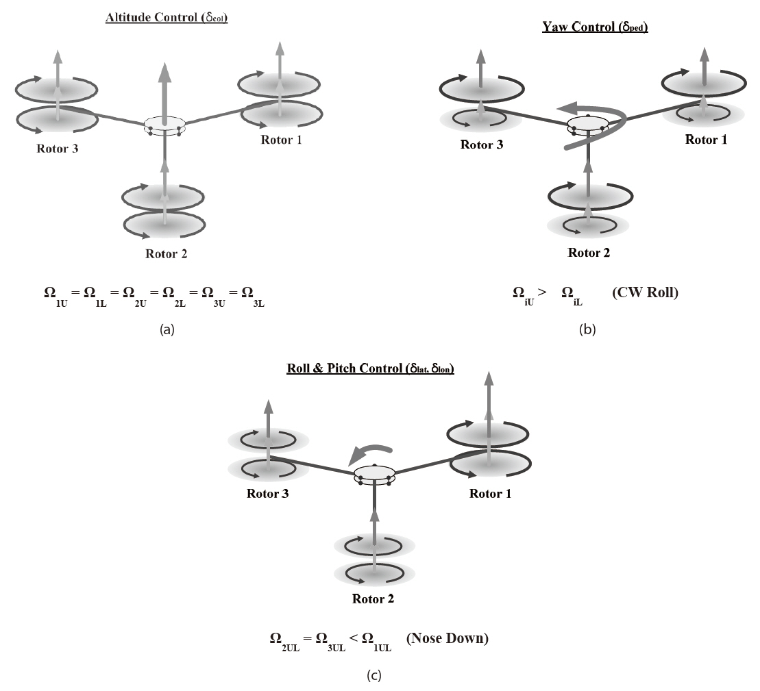
The control strategies of the coaxial tri-rotor show slightly similar methods to those of single tri-rotor UAVs. Figure 6 shows the control strategies of coaxial tri-rotor UAVs.

As shown in Fig. 6, the altitude can be increased by increasing all six rotor speeds at the same time. To perform yawing control, varying the rotor speeds of the upper and lower rotors will create a reaction torque, which leads to a yawing moment. Finally, roll and pitch commands could be accomplished by increasing the upper and lower rotors of

the tail rotor (whichever rotor pairs are located at the back),which would lead to a nose-down pitching moment and vice versa. Rolling is done similar to pitching.

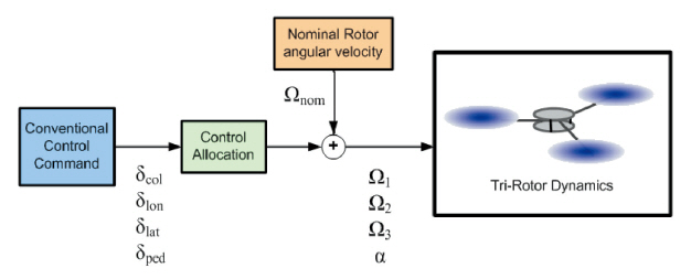
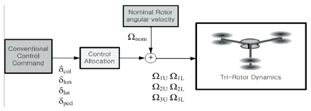
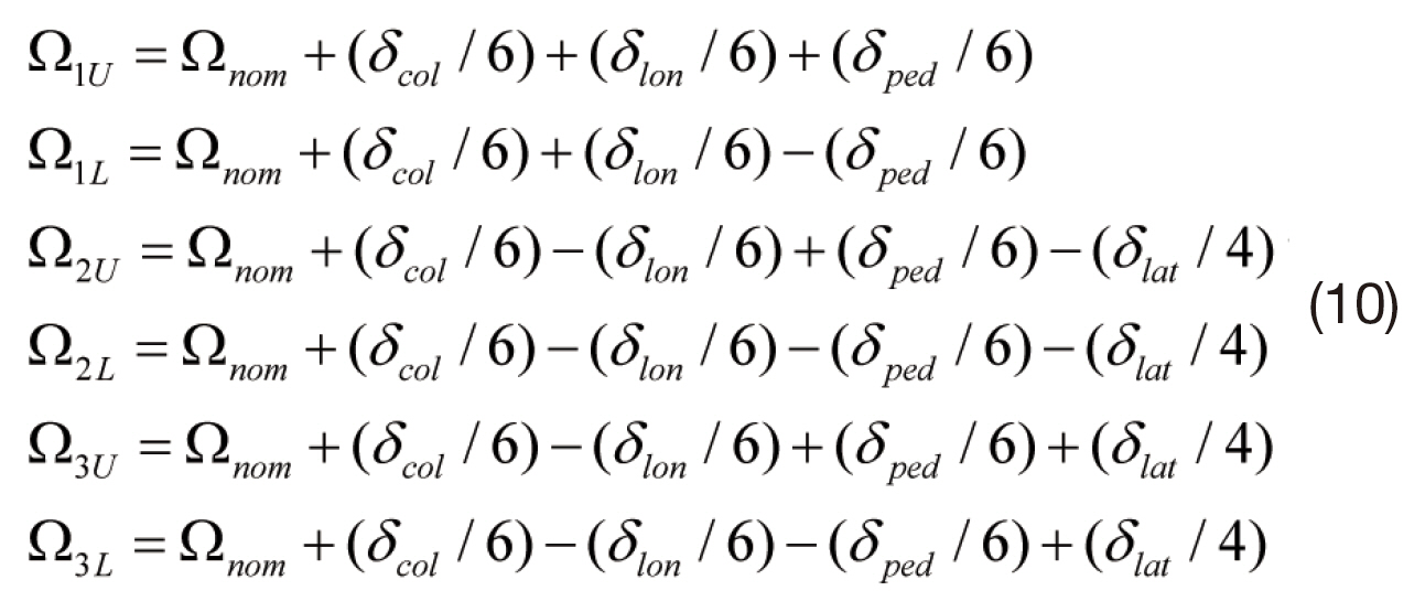
A similar technique from the single tri-rotor’s control system design is applied for the coaxial tri-rotor’s control system design. There are also four command inputs allocated to six rotors. Figure 7 and Eq. (10) describe the control

allocation of the coaxial tri-rotor UAV. The block diagram for the attitude hold autopilot of the coaxial tri-rotor is similar to that of the single tri-rotor, which is represented in Fig. 4.

In this section, numerical simulations for the stabilization of both types of tri-rotor are reported in order to observe the behavior of UAVs in each channel under given command inputs. All simulations were done through MATLAB Simulink.

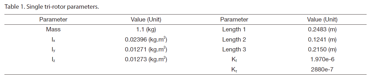
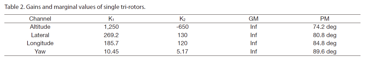
Table 1 shows the parameters of single tri-rotors that are used for the nonlinear simulations. Also, all the gain values used for this simulation and the gain and phase margins from the Bode plots are tabulated in Table 2.

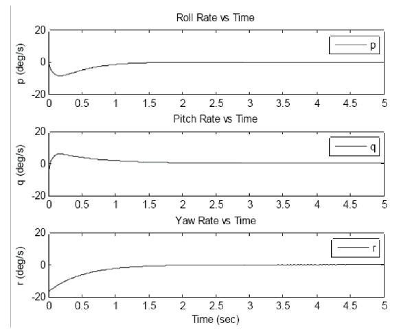
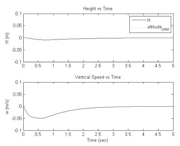
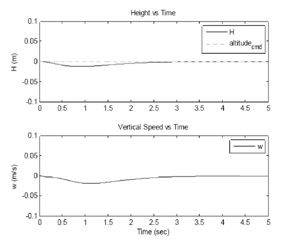
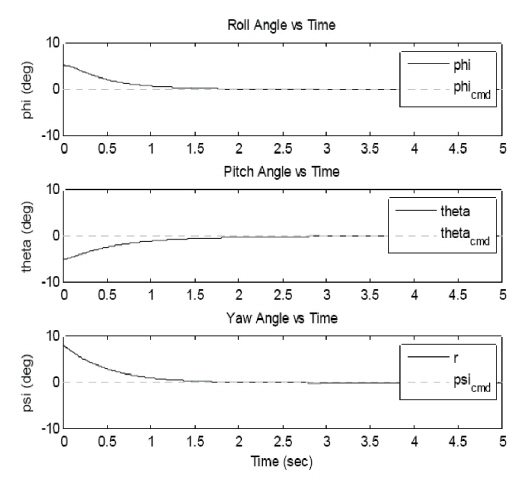
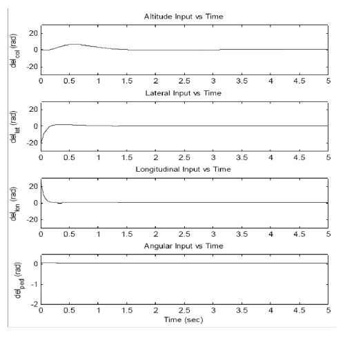
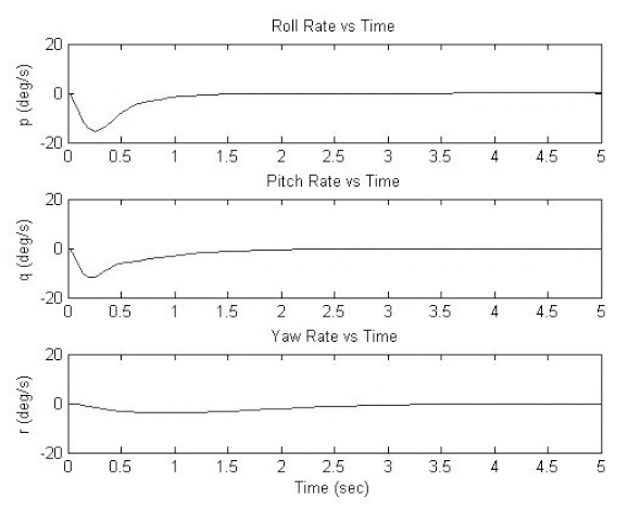
Every gain margin goes to infinity, meaning every channel shows stable behavior. As before, K1 and K2 stand for the rate feedback gains and position feedback gains,respectively. The negative altitude gain K2 comes from the reversed coordinates in the north-east-down (NED) body frame. Every simulation was done for five seconds. The altitude and vertical velocity responses are shown in Fig. 8,and all the angular rate responses are shown in Fig. 9. Figure 10 shows the Euler angle responses, and Fig. 11 shows the control commands. The rising time and settling time were set between one and two seconds for each channel, and overshoots were set close to zero. According to the results

shown in Figs. 8 to 11, it is remarkable that the responses converge to zero after a short amount of time (about 1-2 seconds). Especially in Fig. 7, all the Euler angle responses indicate that even when the initial angles were non-zeros,they converged to zero meaning that attitude control was properly performed. In most of the graphs, there are several“bumps,” and these bumps are from the tilt angle α from the beginning. After about 1-2 seconds, plots tend to return to their original trimmed values. Therefore, these plots show that the attitude and altitude control of single tri-rotor UAVs are possible.

For the coaxial tri-rotor simulations, all the parameters were identical to those for the single tri-rotor except that all the lengths defined in the coaxial tri-rotor configuration were identical to length 1, as shown in the figure for single tri-

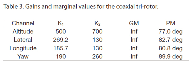
rotors. However, the gain settings of the coaxial tri-rotor for the simulation were slightly different from the gain settings of the single tri-rotor. These are tabulated in Table 3 as well as each channel’s gain and phase margins.

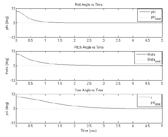
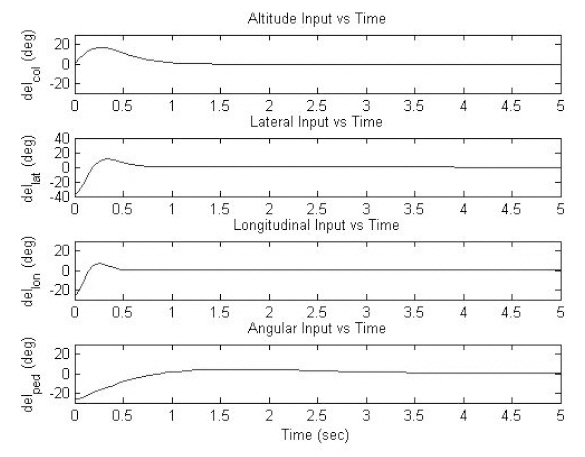
All the gains set for the simulation were aimed for the values between one and three seconds of the rising time and settling time without any overshoot. Figures 12 through 15 respectively display the simulation results for the altitude

and vertical velocity responses, angular rate responses,Euler angle responses, and control commands regarding the coaxial tri-rotor UAV.

Every simulation was performed for 5 seconds. In the figures above, the altitude and attitude channels successfully show their responses as originally assumed: the rising and the settling time were to be between one and three seconds with no overshoot. In Fig. 14, the attitude plots show that the initial commands were given as eight degrees regarding the roll, pitch, and yaw channels, and after a fair amount of time,they all converged to zero degrees. These results denote that the UAV regains its stability even when it has commenced from an unstable position.

In this paper, the importance of a small-sized vertical take-off and landing (VTOL) UAV for various missions was mentioned, and tri-rotor UAVs were introduced as one of the examples. In order to solve the yawing moment problem that the tri-rotor has originally had, two types of tri-rotor UAV are introduced in this paper: single and coaxial. The single tri-rotor UAV solves the yawing moment problem by tilting the tail rotor by the angle α. The coaxial tri-rotor solves the same problem by installing two counter-rotating rotors,which cancel each other’s reaction torques, on each axis. For both types of tri-rotor UAV, attitude and altitude stabilization is necessary, and nonlinear simulations were carried out in order to observe the stability of both UAVs. The simulation results showed that the altitude and attitude responses follow the commands with reasonable rising times and settling times. After observing the simulation results, it is concluded that altitudes and attitude stabilization for both types of trirotor are accomplished properly.