One approach to autopilot design that achieves the effect of gain scheduling is the use of dynamic model inversion (DMI). However, this approach does not eliminate the need for accurate aerodynamic data. In this paper we considered the addition of an adaptive element, on-line neural networks (NNs), in order to help control and eliminate errors incurred when using an approximate model. Also the output redefinition and the two-loop design approach were considered as a means for solving the inverting problem of a non-minimum phase system.

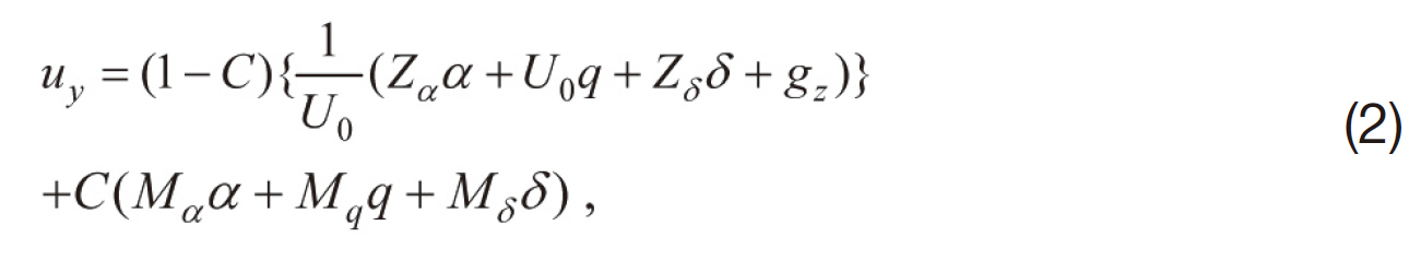
Feedback potentially accommodates uncertainty in order to meet system performance specifications. However, uncertainty can also affect the stability properties of a closed-loop control system. The design of a feedback controller should therefore be based not only on a particular model, but also on the uncertainty in the particular model so that the uncertainty can be quantified. The importance of robustness has long been recognized and tools known as stability margins were developed to quantify it. However, the traditional stability margin analysis techniques based on the linear control theory cannot be applied to the control system to which a representative non-linear control method, such as the NN, has been applied. This paper presents a stability margin technique for a NN applied control system.

Although the design of the controller and simulations are based on a nonlinear 6 degree of freedom model, including longitudinal, lateral and directional channels, this paper does not present the results of the lateral and directional channels for the purpose of conciseness.

Accurate aerodynamic data is necessary for designing a reliable controller that meets practical requirements. It increases developmental time and costs due to the need for additional processes such as wind-tunnel testing and gain scheduling. One alternative method for reducing time and cost is employing an adaptive control. This paper applies DMI with NN eliminating inversion errors (Kim and Calise, 1997; Sung and Kim, 2007). This approach greatly reduces the procedure and time in comparison to classical gain scheduling because it uses DMI at a single flight condition.

A drawback to DMI is that it cannot be applied to nonminimum phase plants. Unfortunately, transfer functions from control surface to acceleration (at the center of gravity) are always at the non-minimum phase for tail mounted surfaces. Thus, dynamic inversion cannot be used to directly control acceleration. The non-minimum phase problem can be avoided by first designing an inverting controller for a transfer function that is at the minimum phase, and then adding a classically designed outer loop around it. The problem with this approach is that the transfer function from the control surface deflection to the body rate has a zero very close to the origin, the effect of which is to produce a very slow mode when the inversion is inexact. This slow mode potentially causes difficulty in meeting design criteria, such as rise time and settling time. A second possibility is to control the aerodynamic angles in the inner loop. This approach avoids the problem of a slow mode in rate design, but results in a zero far in the left half plane. As a result, rapid transients occur in the control response. Moreover, this approach was later found to be sensitive to time delays (Calise et al., 1998).

This paper uses an alternative approach called output redefinition for plant inversion of a tail controller missile. This approach allows the designer to place the zero of the associated transfer function at a desirable location. The design for the longitudinal channel applies a classical twoloop design, with acceleration regulated in the outer loop. Since a non-minimum phase plant cannot be inverted directly, the two-loop design avoids the non-minimum phase problem by first applying an inverting controller for a transfer function that is at the minimum phase, and subsequently adding a classically designed outer loop around it. The outer loop employs both proportional and integral gains (Calise and Sharma, 1998; McFarland and Calise, 1997; Ryu et al., 1997).

The directional channel architecture is identical to that of the longitudinal channel. The lateral channel implementation is much simpler because the transfer function from fin deflection to roll rate contains no finite zeros. The directional and lateral channel architectures are not presented in here.

The output redefinition, a blend of angle of attack (α) and pitch rate (q),

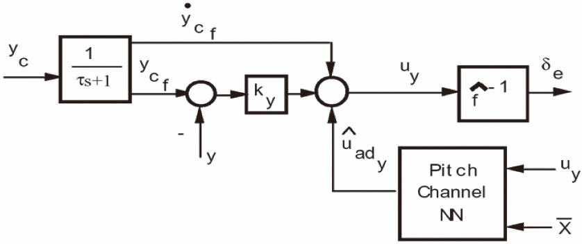
is used for the inverting inner loop because the transfer function from elevator deflection to y has zeros in locations more favorable than those corresponding to either α or q alone. A block diagram of the inner-loop architecture is shown in Fig. 1.

Dynamic inversion is based on the redefined output variable, y. Differentiating Eq. (1) and using the linearized longitudinal equations results in the following approximate expression for the inverse

where u_y is the corresponding pseudo control (desired rate of change y). The gain k_y is used to regulate the error transient, and is chosen to be sufficiently large to insure that the error transient is fast compared to the time constant, τ. A reasonable choice is k_y =3/τ (Calise and Sharma, 1998).

The purpose of the NN is to account for errors in the approximate inverse of the transfer function from the elevator deflection to y. If the NN successfully eliminates the effect of errors, and perfect inner-loop tracking is achieved following a brief transient period. Pseudo control hedging is also applied to the inner loop working in order to reduce the influence of time delays caused by the actuator and actuator saturation.

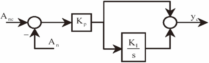
The outer loop is used to regulate acceleration, and generates a command signal to the inner loop. Feedback

inversion with output redefinition is then applied in the inner loop. The outer loop portion is illustrated inFig. 2.

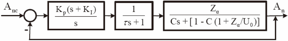
Assuming perfect inner-loop tracking in combination with the assumption,

results in the idealized outer-loop diagram illustrated inFig. 3.

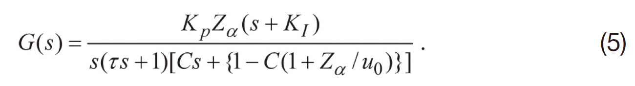
The open loop transfer function of the idealized loop is given by in Eq. (5).

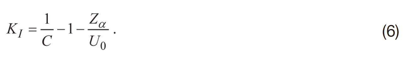
K_I is given in Eq. (6) and is selected for pole-zero cancellation.

Then, the transfer function of the closed loop system is

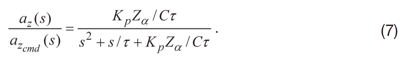
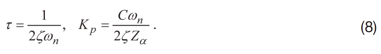
From Eq. (7) the natural frequency and damping ratio of the closed-loop system can be determined by selecting

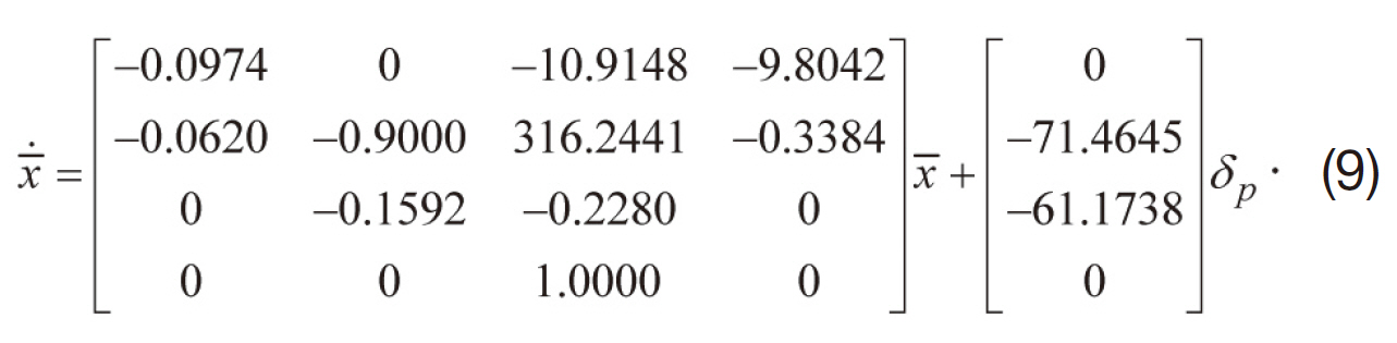
The aerodynamics of a missile was obtained from Missile DATCOM. The specifications of the applied missile are as follows: length: 4.69 m; diameter: 0.35 m; weight: 670 kg; thrust at cruise speed: 3,650 N. The following state space equation, Eq. (9) is the linear dynamics at a single flight condition in which Mach 0.93 is the cruising speed, and where δ_p is the pitch effecter.

Actuator dynamics is modeled as a first order system with a 0.01 sec time constant. The rate limit and deflection limit were ±600 deg/s and ±30 deg, respectively.

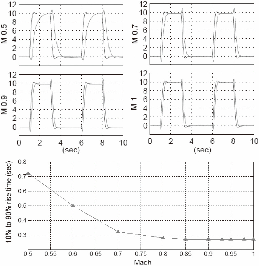
A 10%-to-90% rise time specification was used as the performance specification in this application. This criterion removed the effect of the time delay. The applied rise time specification was 0.3 seconds. The outer loop control parameters were selected to a damping factor of 0.8, C, the coefficient of the output redefinition of 0.3, and a variable natural frequency increasing along the speed.

The rise time performance across the flight envelope is shown in Fig. 4. It shows that the rise time requirement was satisfied above Mach 0.75. Low dynamic pressure was the primary reason for the degradation of rise time performance in the low speed range. Although the stability and control augmentation systems of the missile can not meet the requirement for the whole flight envelope, it seemed acceptable considering the cruise speed was around Mach 0.93.

The stability margins were used as the measurement of the robustness of the closed-loop system with respect to model

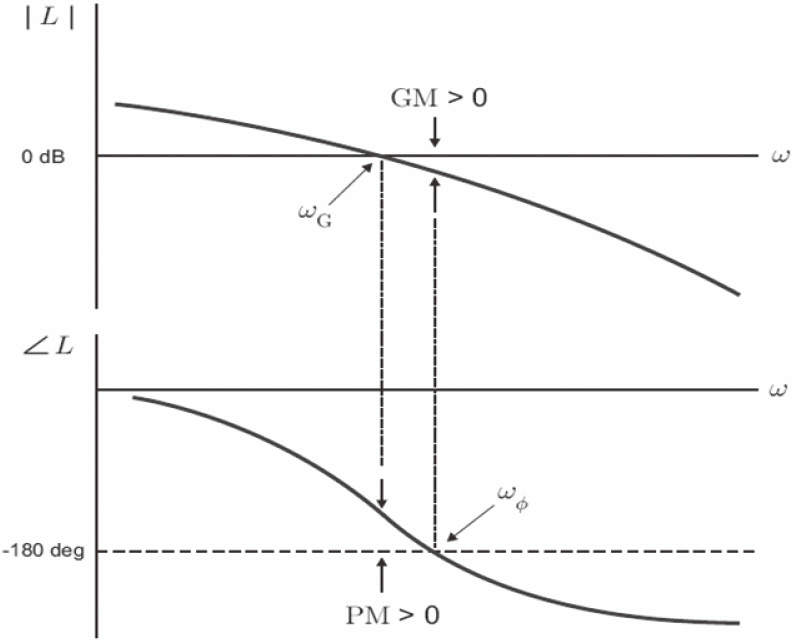
uncertainties. In classical control theory, two commonly used quantities are the gain margin (GM) and the phase margin (PM) defined in terms of the loop gain L(s). Figure 5 illustrates the GM and PM of a closed-loop system using Bode diagrams of the open-loop systems.

The GM and the PM may also be defined in terms of the Nyquist plot from the measures of how close the Nyquist plot comes to the point -1+j0. The GM can also be determined from a root locus by using the ratio of the gain at which the root locus crosses the imaginary axis to the gain at the nominal closed loop poles.

In general, either the GM or the PM alone does not give a full indication of the robustness of the closed-loop system. One should examine both quantities in order to describe the robustness. For a satisfactory design, the phase margin was usually chosen to be between 30° and 60°, and the gain margin to be greater than 6 dB.

The GM and PM of the traditional stability margin are based on the linear time-invariant theory. The GM and PM of the closed loop system can be read directly from the Bode plot or Nyquist plot of the open-loop system, as previously stated.

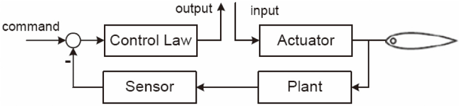
For the open-loop transfer function, a feedback loop of one control system axis remained opened. Figure 6 shows the relationship between the elements described above and where input and output signals are located. The loop is shown opened just upstream of the actuators but it can be opened anywhere in the loop as long as all major contributing paths are represented at the break.

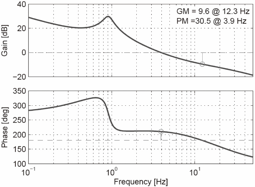
Figure 7 shows the stability margins in the longitudinal axis of the designed anti-ship missile control at the flight condition of Mach 0.8, directly from the Bode plot.

The method used to calculate the stability margins described above use open loop transfer functions based on linear control theory.

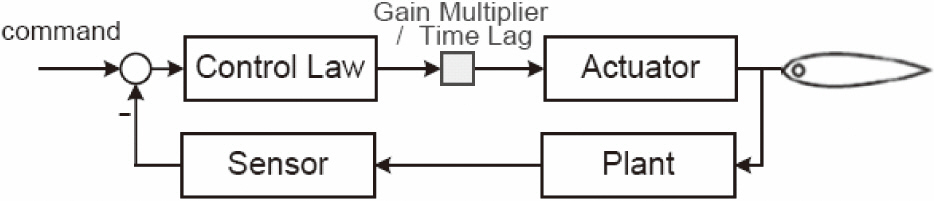
Difficulty arises when applying an open loop transfer function of a control system to a representative non-linear control method, NN. This problem can be solved by extending the concept of the stability margin calculation from the root locus. The root locus was used to study the effect of loop gain variations. Upon suggestion, we plotted the locus of all possible roots of Eq. (10) as K varied from zero to infinity and then used the resulting plot to aid us in selecting the best value of K.

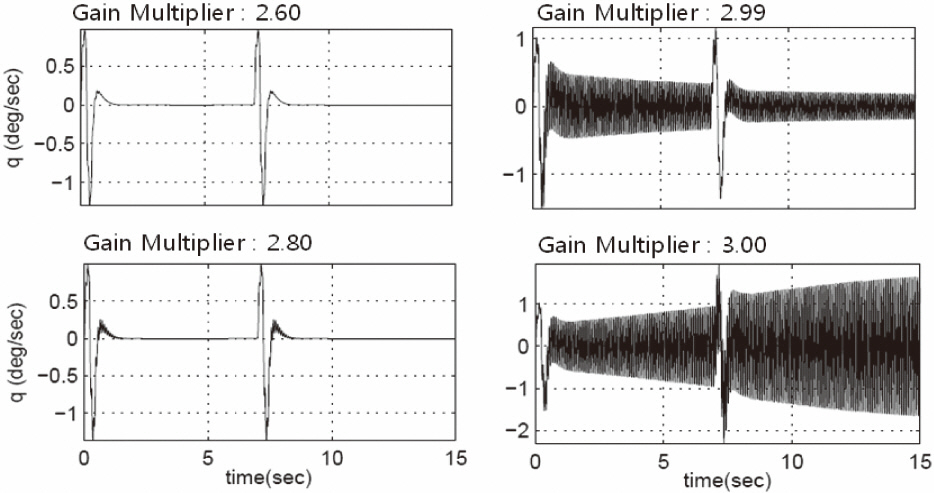
The above mathematical expression can be interpreted as adding the gain multiplier K to the closed loop and then monitoring the system response for the increased gain multiplier. This concept is illustrated in Fig. 8.

In general, as the value of the gain multiplier increased, the system response changed from stable to neutral stable and then to unstable. In this approach, the gain in neutral stable was the gain at which the root locus crossed the imaginary axis.

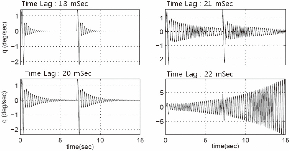
In the same way, we added the time lag element to the closed loop, reviewed the response and increased the time lag, and found the value of time lag in neutral stable. And, we calculated the PM by the following relation.

The method, a stability margin calculation by using the simulation response, was commonly used to validate the stability robustness of the control system in a hardware-inthe-loop simulation phase.

Figure 9 shows the responses of an anti-ship missile to the pitch command along the increased gain multiplier. Two pitch double commands were inserted in consideration of a brief transient period of the NN. The same pitch doublet command was used for all the responses in this paper. From Fig. 9, we expected to find that the value of the gain multiplier in neutral stable form was within the range of 2.99 and 3, Indicating that the GM of the closed loop system was around 9.53 dB ( =20log₁₀2.995/1).

Figure 10 shows the responses to the pitch command along the increased time lag. We expected to find the value of the time lag in the neutral stable case from the responses.

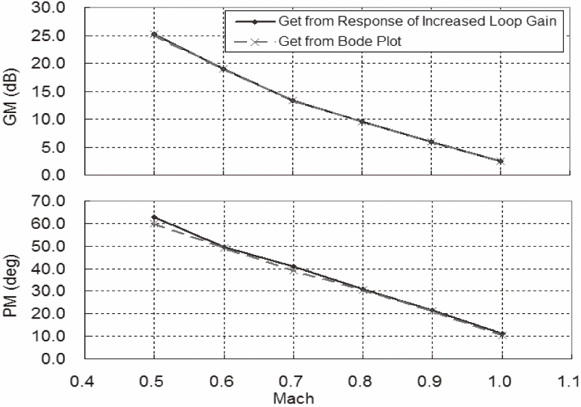
Figure 11 illustrates the comparison of stability margins between the calculation from the simulation responses and the read value from the Bode plot. We disengaged the NN of the inner loop for comparison purposes. Figure 11 shows that stability margins from the simulation responses matched well the responses provided by classical theory.

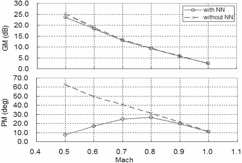
Figure 12 illustrates the comparison of stability margins between the conditions of NN engaged and those of NN disengaged.

Both stability margins were calculated from the simulation responses. We disengaged the NN of the inner loop for comparison purposes. Although both GMs were similar, the PM from the disengaged NN was less than that

from the engaged NN, especially in the low speed range. The main reason for this difference is that the slow dynamic characteristics were used for the input of NN. Although we considered the following general observations: the phase drops off rapidly with increasing frequency; and, a physical system for which the transport lag has been neglected will have a phase that is strictly less than predicted (Franklin et al., 2002), the low phase margin needed to be improved. The authors plan to improve the stability margins by the tradeoff between performance and stability using the similar

way mentioned the Section 3.4 and the study applying the actuator which has faster dynamic characteristics.

In many practical applications, the compensator design is essentially a compromise between performance and robustness. This trade-off in the anti-ship missile control design is presented here.

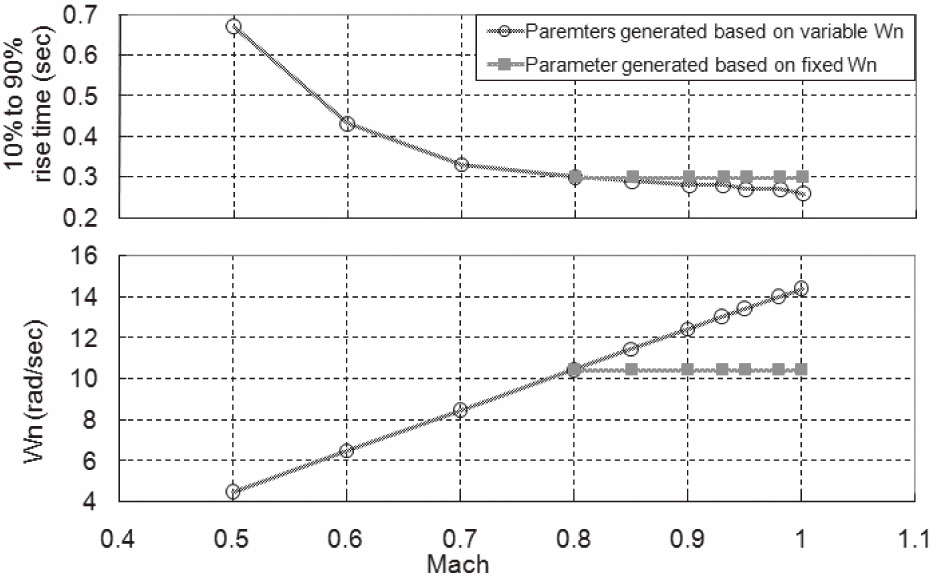
Figure 13 shows a 10%-to-90% rise time performance degradation when the control parameters calculated based on a fixed natural frequency were used in the speed range above Mach 0.8. Although there was a degradation of the rise time performance in the specific speed range, it still met the 10%-to-90% rise time specification. Thus, the study of a trade-off between the degradation of rise time and the stability margin has been performed.

Figure 14 shows the enhancements of the stability margin by applying the control parameters, taking into account the degradation of the rise time performance.

A NN based adaptive inverting control design was developed and evaluated for an anti-ship missile. The design,which used data for a single flight condition, resulted in acceptable performance across the flight envelope without gain scheduling. The potential to reduce the dependence on accurate aerodynamic data was presented.

The stability margin analysis technique for the neural network applied system was presented. It used the simulation responses of the control system inserted gain multiplier or time delay element. Results also showed the possibility of enhancement in stability margins by accounting for acceptable degradation of performance.