An integrated system composed of guidance, navigation and control (GNC) system for autonomous proximity operations and the docking of two spacecraft was developed. The position maneuvers were determined through the integration of the statedependent Riccati equation formulated from nonlinear relative motion dynamics and relative navigation using rendezvous laser vision (Lidar) and a vision sensor system. In the vision sensor system, a switch between sensors was made along the approach phase in order to provide continuously effective navigation. As an extension of the rendezvous laser vision system,an automated terminal guidance scheme based on the Clohessy-Wiltshire state transition matrix was used to formulate a “V-bar hopping approach” reference trajectory. A proximity operations strategy was then adapted from the approach strategy used with the automated transfer vehicle. The attitude maneuvers, determined from a linear quadratic Gaussian-type control including quaternion based attitude estimation using star trackers or a vision sensor system, provided precise attitude control and robustness under uncertainties in the moments of inertia and external disturbances. These functions were then integrated into an autonomous GNC system that can perform proximity operations and meet all conditions for successful docking. A sixdegree of freedom simulation was used to demonstrate the effectiveness of the integrated system.
Autonomous rendezvous and docking are important technologies for current and future space programs, including missions such as supply and repair to the International Space Station (ISS) and the exploration of the moon, Mars, and beyond. Proximity operations and docking require extremely delicate and precise translational and rotational maneuverings. During the final approach of the proximity operations phase, the relative position,velocity, attitude and angular rates between the target and the chaser spacecraft must be precisely controlled in order to obtain the required docking interface conditions. As a consequence, precise relative position, velocity and attitude state estimations are required. The first spacecraft rendezvous and docking dates back to the manned US Gemini and Apollo programs (Zimpfer et al., 2005) and the unmanned Russian Cosmos missions of the late 1960s. The Apollo program, even with limited computer resources, demonstrated many of the guidance, navigation and control functions required by current autonomous rendezvous and docking procedures. As the next step to the Apollo program, the Space Shuttle (Zimpfer et al., 2005) program, which began in the early 1980s, has demonstrated rendezvous and docking functions for various types of spacecraft. The onboard shuttle guidance, navigation and control (GNC) system with crew command can automatically perform various rendezvous functions including translation and rotational control, targeting, and relative navigation. However, the crew manually performs the final approach maneuvering phase within about 90 meters of the target using visual images from the centerline camera fixed to the center of the orbiter’s docking mechanism, the trajectory control sensor, and laptop situational awareness displays. Since the early 2000s, there have been several programs proposed to demonstrate the capabilities of autonomous rendezvous and docking. The demonstration of autonomous rendezvous technology (DART) mission (Rumford, 2003) provided a key step in establishing autonomous rendezvous capabilities for the US space program by performing autonomous rendezvous. The orbital express program (Gottselig, 2002) aimed to demonstrate several satellite servicing operations and technologies including rendezvous, proximity operations and stationkeeping, capture, docking, and fluid (hydrazine) transfer. The Experimental Satellite System (XSS) series (Zimpfer et al., 2005) conducted by the US Air Force demonstrated increasing levels of microsatellite technology maturity such as inspection, rendezvous and docking, repositioning and techniques for close-in proximity maneuvering around orbiting satellites. Semi-autonomous operations and visual inspection in close proximity of an object in space were demonstrated. The automated transfer vehicle (ATV) (Fabrega et al., 1996; Gonnaud and Pascal, 1999; Pinard et al., 2007) is an expendable, unmanned resupply spacecraft developed by the European Space Agency (ESA). The ATV program is designed to perform automated phasing, approach, rendezvous and docking to the ISS, followed by departure and deorbit maneuverings. It uses absolute and relative global positioning system (GPS) navigation and a star tracker to automatically rendezvous with the Space Station. At a distance of 249 m, the ATV computers use videometer and telegoniometer data for final approach and docking maneuvering. The actual docking to Zvezda,the Russian service module on the ISS, is fully automated.The first Jules Verne ATV mission was launched on March 9,2008 and docked successfully to the ISS on April 3, 2008. The elements composing the ATV nominal rendezvous strategy include a drift phase, homing transfer, closing transfer, and final translation.
The need for a fully autonomous GNC system to fulfill rendezvous missions is still in demand. The minimum objective of this study is to propose an integrated system composed of GNC system based on linear quadratic Gaussian (LQG)-type controls and then, demonstrate the capability of the autonomous GNC system for the newly adapted approach strategy. For this demonstration, the approach strategy of the ATV translating to the V-bar docking port was selected among the space programs discussed above and modified as a case-study to evaluate the integrated autonomous GNC system developed in this study. The original approach strategy of the ATV was not directly utilized but modified to extend the range of the rendezvous laser vision (RELAVIS) (Pelletier et al., 2004) scanning system. The integrated system can then span the close-range rendezvous phase which is beyond the proximity operations range. As a result, the integrated system could be extended to deep space where GPS system was not available. This was made possible by using an intercept guidance scheme based on the Clohessy-Wiltshire (CW) state transition matrix propagation, leading to a possible application of RELAVIS. The integrated system demonstrated the capability required for various translational and rotational maneuvers in the proximity operations phase through a six-degree-of-freedom simulation and met the final conditions required during the docking phase.
2. Overall Proximity Operations Strategy
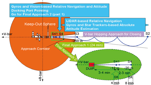
A new proximity operations strategy adapted from the ATV approach strategy using an alternative navigation system (the RELAVIS scanning system) was investigated in this study. The field of view (FOV) that resulted from the geometry of the ATV’s “V-bar hop” closing transfer exceeded the FOV constraints required by the RELAVIS system. For this reason, the closing approach was modified to a V-bar hopping approach developed in this study so that the FOV requirements could be satisfied, allowing the use of the RELAVIS system. The proximity operation operations strategy proposed here is illustrated in Fig. 1. The case study scenario considered here begins from location S2, the beginning point of the closing transfer. The various phases of this closing transfer include: V-bar hops from S2 to S3, stationkeeping at S3, straight line approach from S3
to S4, a second period of stationkeeping at S4, straight line approach from S4 to S41, a third period of stationkeeping at S41, and a straight line approach from S41 to the docking port. The proximity operation strategy is conducted step-bystep in a predefined manner. Relative GPS (RGPS) used in the ATV approach strategy was replaced with the RELAVIS scanning system for the interval from S2 to S41. Videometerbased relative navigation used by the ATV was replaced by the more accurate RELAVIS vision-based navigation for the interval from S4 to the docking port in order to meet the strict requirements of the approach corridor. Also of importance was a 200 m spherical area surrounding the target called the “Keep-Out Sphere.” This volume can be entered only through one of the approach and departure corridors. No vehicle is allowed to penetrate this space except through the circular cone (Pinard et al., 2007).
The GNC system performed this new proximity operations strategy without direction from a terrestrial ground station. The GNC system autonomously selected the navigation system used along the various phases and determined the control commands using the predefined guidance function and the real-time onboard navigation function.
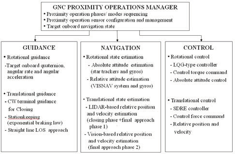
3. GNC Proximity Operations Architecture
The proposed GNC system was composed of independent GNC functions, managed by a centralized GNC processor. Figure 2 provides an overview of the GNC proximity operations architecture. The GNC proximity operations manager covered functions common to GNC, including command, data handling, and managed overall mission phase sequencing. Because of the many different maneuver and navigation requirements, and the variety of attitude and navigation sensors used in the various proximity operations phases, a different set of algorithm parameters and hardware
functions was used in each phase. The guidance function provided the predefined reference trajectory and transferred the target’s attitude and angular rate through onboard communication to the controller. When simulating the closed-loop GNC system, the high precision orbit propagator in the Satellite Tool Kit (STK) (Analytical Graphics Inc.) was used to produce the target’s inertial position and velocity vectors.
The quaternions that defined the orientation of the target vehicle with respect to the inertial frame and the target’s angular rate expressed in the body-fixed frame of the target vehicle were also simulated. The navigation function estimated the relative position, velocity, absolute and relative attitude. This 13-dimensional target vector was assumed to be available through onboard navigation and was provided to the GNC functions by the GNC proximity operations manager. The control function determined the forces and torques necessary for tracking the desired state provided by the guidance function. During the proximity operations, various translational and rotational maneuvers were executed using input from different sensor types. The combined set of algorithms and parameters used to execute maneuverings was termed the GNC module. The GNC module consisted of a set of GNC modes. The guidance function provided the reference states working as feedforward terms in the controllers. The navigation function estimated the relative position, velocity and attitude onboard the spacecraft. The estimated states were then combined with the optimal controllers by replacing the control state with the estimated state.
4.1 Translational relative motion dynamics
The chaser’s relative motion dynamics including the Earth oblateness effect J2 and aerodynamic drag was first provided. Among the many sources of perturbations between the target and chaser, Earth oblateness and aerodynamic drag in low earth orbit were dominant and were included in the nonlinear relative equations of motion. In the CW frame E, the perturbing acceleration due to J2 (Prussing and Conway, 1993) was quantified by
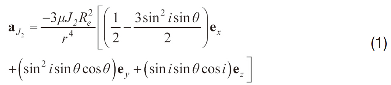
The relative effect of Earth oblateness due to J2 then becomes
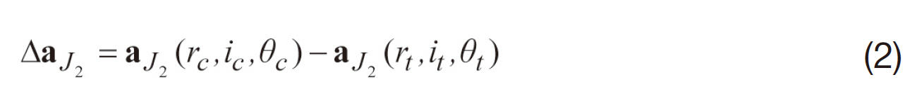
where subscripts t and c denote the target and the chaser,respectively. The perturbing acceleration in the CW frame due to aerodynamic drag was computed by expressing the acceleration in terms of the Earth centered inertial frame (Vallado and McClain, 2001). The relative effect of atmospheric drag in the CW frame is then

Where, C is the 3-1-3 rotation sequence C=C3(θc)C1(ic)C3(Ωc). Thus, the sum of the relative effect of Earth oblateness and drag becomes

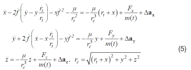
Consequently, the equations of motion for the translational control formulation becom
4.2 Rotational motion dynamics and kinematics
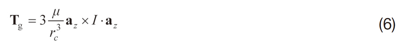
The rotational motion of the chaser was expressed in the body-fixed frame using the well-known Euler’s equations of motion. Like the perturbing accelerations in relative motion dynamics, rotational motion dynamics also experienced disturbing torques such as torque due to aerodynamic drag, magnetic field torque, and gravity-gradient torque due to spacecraft asymmetry. This study only modeled the gravitygradient torque. The effects of the gravitational field were not uniform over an arbitrarily shaped body in space, creating a gravitational torque about the body’s center of mass. This gravity-gradient torque, expressed using the local orbital frame A, is given in vector/dyadic form Wie (1998) as
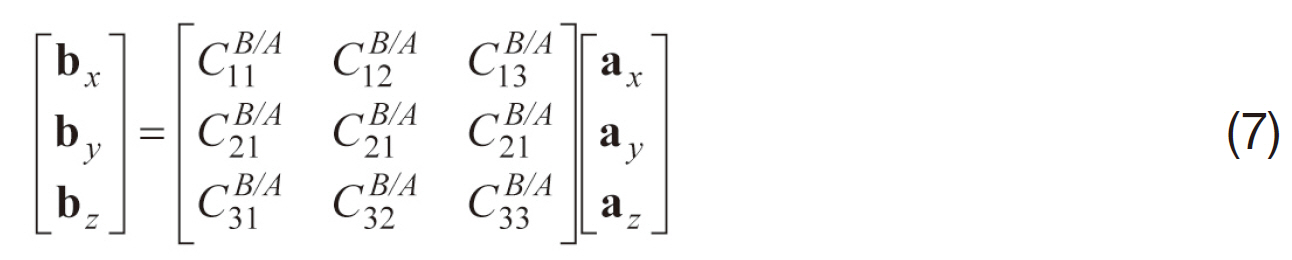
The orientation of the body-fixed frame B of the chaser with respect to the spacecraft local orbital frame A of the chaser is described by the direction cosine matrix CB/A as
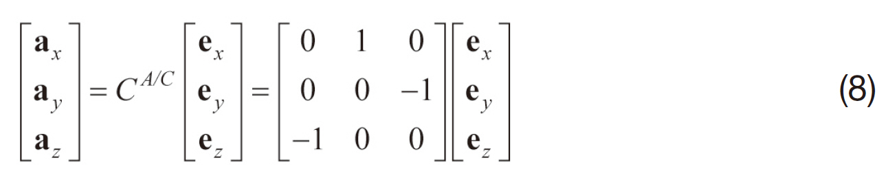
The orientation of the local orbital frame A of the target spacecraft with respect to the CW frame C is described by the direction cosine matrix CA/C such that
The direction cosine matrix CB/A can be expressed using successive rotations with the inertial frame N through CB/A=CB/NCN/A. The angular velocity of the chaser, ω= ωB/N and az can be expressed in terms of the basis vector of the bodyfixed frame B of the chaser as


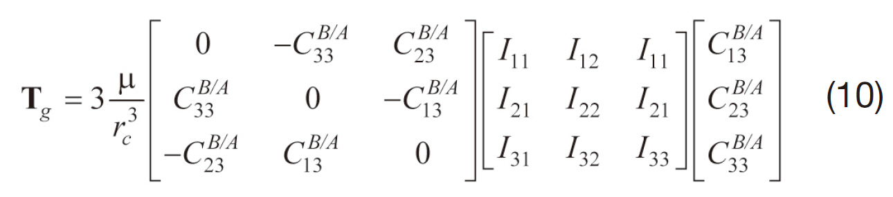
The gravity-gradient torque becomes
A full description of the rotational motion of a rigid spacecraft requires both kinematic and dynamic equations of motion. For most modern spacecraft applications, quaternion kinematics (Lefferts et al., 1982) are preferred. The quaternion kinematic equation of the chaser is

where
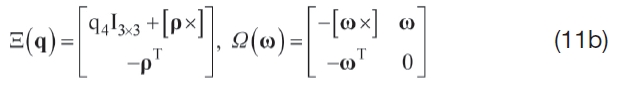
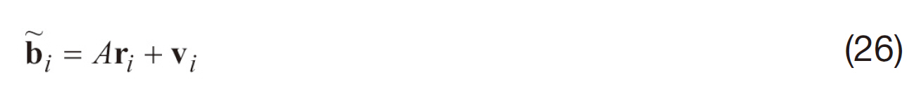
The adopted quaternion27 is defined by
where ρ is defined as [q1 q2 q3]T=esin( ?/2), and q4=cos( ?/2) Euler’s rotational equation of motion, including the gradient torque, is given by
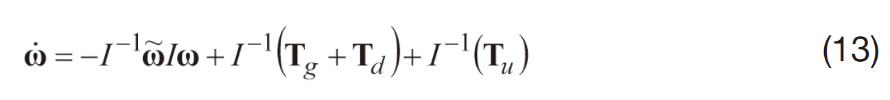
where Td is modeled by white Gaussian-noise
The guidance function provides both translational guidance and rotational guidance. The translational guidance determines commands designed to bring the chaser to a desired velocity. An automated terminal guidance scheme based on the CW state transition matrix is used to provide the reference trajectory for the closing transfer composed of three V-bar hops. The transfer time and required ΔV in the closing phase are also determined. The general solution can be conveniently expressed in terms of the state vector

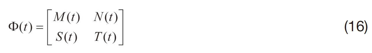
by means of its 6×6 state transition matrix Φ(t) (Prussing and Conway, 1993) for which

where the lower-case Greek “deltas” indicate relative quantities between the chaser and target vehicles. The state transition matrix Φ(t) is partitioned into four 3×3 partitions as
The necessary chaser initial (relative) velocity with which to intercept the target at the final time is obtained by
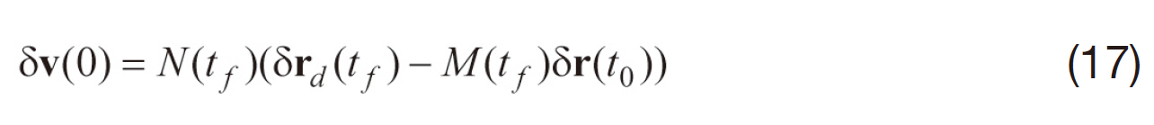
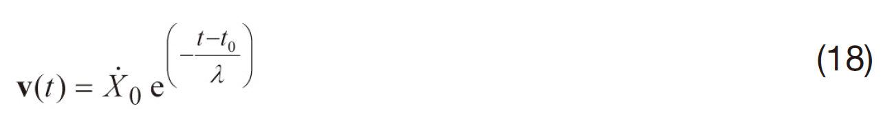
The reference state is then propagated using Eq. (15) with computed initial velocity in Eq. (17). After the closing transfer reached S3, stationkeeping was then performed for four minutes at S3 and was again performed at S4 and S41 after V-bar straight line maneuverings. The required settling time for the stationkeeping phase was predetermined using the exponential braking law and control techniques (described below). This setting time can be varied to accommodate the autonomy of the GNC system if a longer time was required for the stationkeeping phase. When the stationkeeping initiated, the chaser vehicle followed bounded relative motion in three-dimensional space. The stationkeeping phases at S3, S4, and S41 maintained the desired constant position and zero velocity. Since the vehicle arrived at S3 with nonzero velocity, retro-firing of thrusters was required. To nullify the arrival velocity, the exponential braking law (Paielli and Bach, 1993), characterized by an exponential change of velocity with time, was specified as
After the stationkeeping phases, straight-line forcedmotion trajectories were used for the V-bar final approaches with constant velocity from S4 to S41 and from S41 to the docking port. This type of trajectory implemented a constant relative velocity of Vx=(x(t)-x(0))/t with respect to the target between the initial x0 and the desired x(t), with the velocity along the other directions maintained at zero. The equation for the reference x(t) along the V-bar direction is simply given by
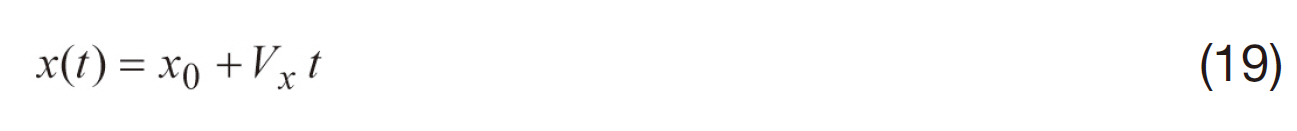
where x(t) at the terminal time becomes zero.
Guidance for rotational maneuvering was provided by onboard navigation and a local communication link. The target’s quaternion, angular rate and angular acceleration became the chaser’s desired ones to track in order to provide the required attitude alignment.
Four different navigation sensor systems were used during the approach phases. The RELAVIS scanning system was used for translational motion, and absolute attitude estimation was made using star trackers. Three axis rate-integrating gyros were also used for attitude estimation. Vision-based relative navigation was used beginning at S4 to provide accurate navigation that satisfied docking requirements. The absolute attitude quaternions can be computed using the quaternion product between the relative quaternions estimated by vision-based navigation and the known target quaternions provided by the target onboard navigation system.
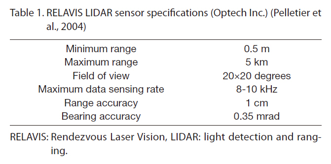
6.1 RELAVIS scanning system-based estimation
The RELAVIS scanning system has the unique capability of producing highly accurate measurements over a range of 0.5 m to 5 km, providing range and bearing (azimuth and elevation angles) of the target with centimeter-level accuracy in range and about 0.02 degree in bearing (Pelletier et al., 2004). The sensor specifications are shown in Table 1.
The range, bearing accuracies, and FOV are of particular interest. Laser range-finder sensors, based on scanning
[Table 1.] RELAVIS LIDAR sensor specifications (Optech Inc.) (Pelletier et al. 2004)

RELAVIS LIDAR sensor specifications (Optech Inc.) (Pelletier et al. 2004)
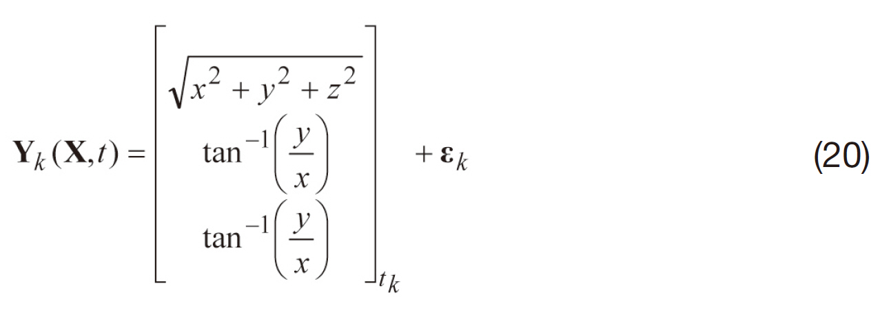
laser radar, have a limited FOV. In order to facilitate the use of RELAVIS, the ATV one-hop V-bar approach during the closing transfer was modified in this study to three hops using the CW terminal guidance so that the nominal approach trajectory met the FOV constraint. The RELAVIS minimum and maximum ranges spanned the line-of-sight angles encountered from S2 to S4. The measurement errors were simulated as white Gaussian noise with zero mean. The bias error was not included because the error was relatively small and was negligible compared to the random errors. The range-angles measurement model, consisting of range, azimuth and elevation angles, is defined by the measurement vector at tk as
The RELAVIS navigation algorithm uses an extended Kalman filter (EKF) filter. The order of the conventional EKF algorithm was modified so that measurement updates would be processed first. The partial derivative matrix for the nonlinear state-space model, omitting the relative perturbation terms for simplicity, is given as
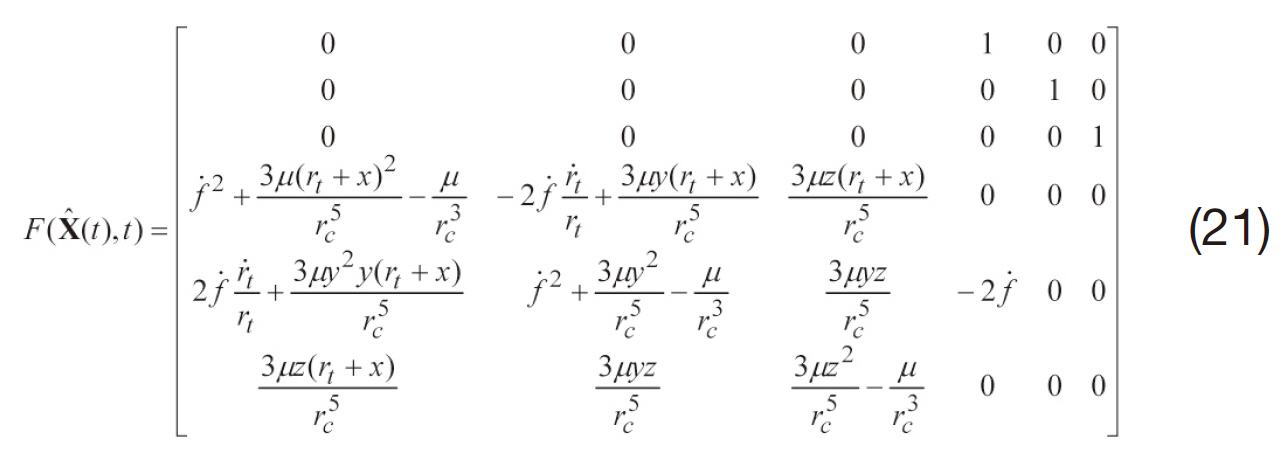
The nonlinear state-space model, X =f(x), followed Eq. (5). The error covariance for the system process noise is given by
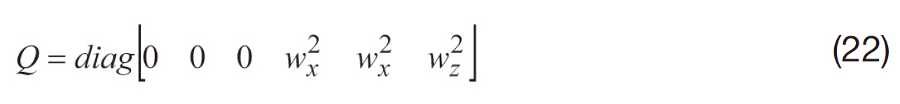
where wx, wy and wz are system process noise. The matrices F and Q were used for covariance propagation. By taking the partial derivative of the measurement vector, the measurement sensitivity matrix at tk is given by
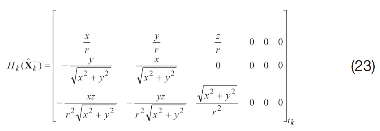
Thus, the EKF filter in the RELAVIS scanning system became capable of estimating the relative attitude, position and velocity.
6.2 Vision-based measurement and gyro models (Junkins et al., 1999)
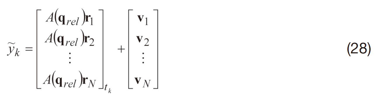
The VISNAV sensor provides line-of-sight (LOS) vectors between the target and chaser vehicles using a small position sensing diode (PSD) that senses beacon light sources. Electronic circuitry controls both the beacons and the PSD sensor. The relationship between the position/attitude and the measurements used in photogrammetry involves a set of colinearity equations, which can be reconstructed in unit vector form as

The measurement equation is then described by
where (x, y, z) are the unknown object space locations of the sensor modeled by Eq. (5). The measurement standard deviation (Kim et al., 2007) is given by 0.0005 degrees. The measurement covariance matrix used in the EKF filter from all available LOS vectors is given by
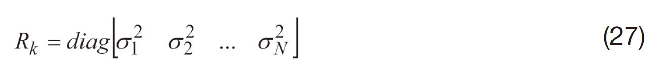
where σi, i=1…N is the measurement standard deviation. Multiple (N) vector observations can be concatenated to
A sensor commonly used to measure the angular rate is a rate-integrating gyroscope, in which a widely-used model is given by


In this study, (ηtv, ηtu) and (ηcv, ηcu) denote the target and chaser gyros, respectively. Gyro measurements are expressed in the inertial frame. The gyro noise parameters are given by σtu=σcu= 10×10?10 rad/sec3/2 and σtu=σcu= 10×10?5 rad/sec1/2 (Kim et al., 2007). The initial biases for each axis of both the target and the chaser gyros are given as 1 deg/hr.
6.3 Vision-based relative attitude estimation
A formulation for the relative attitude estimation, as well as the target and chaser gyro biases, was derived next. The truth equations (Kim et al., 2007) are given as


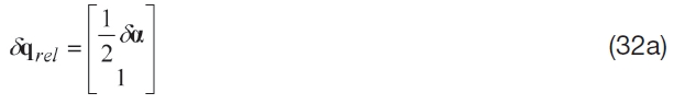
where ⓧ denotes quaternion multiplication. This work adopted the convention of Lefferts et al. (1982) who multiplied the quaternions in the same order as the attitude matrix multiplication. The quaternion qrel describes the relative attitude between the target and chaser. The quaternion inverse is defined by q?1=[?ρ q4]. The relative angular rate is denoted ωct. The error quaternion and its derivatives are given as


where the “hat” symbol “^” denotes the estimated state. For small angles the vector component of the quaternion is approximately equal to half angles and the scalar part of quaternion is equal to one, given by

This study used error-state dynamics that approximated quaternion derivatives for attitude estimation, derived in Kim et al. (2007) as

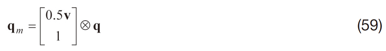
The error-state vector for the relative attitude estimation was augmented to include the relative position and velocity vectors. The error-state equation for the relative attitude estimation was combined with the nonlinear equation of motion in Eq. (5) adding the process noise. The augmented error-dynamics is then expressed by in state-space form as
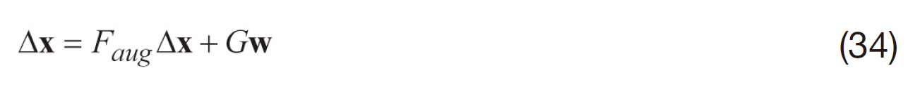


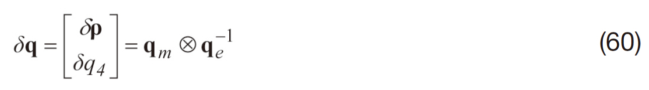
where ΔρT and ΔρT are the error-state vectors for the relative position and velocity estimation. The matrices Faug and G used in the EKF covariance propagation are given by
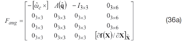
where the partial derivative matrix, ? f(x)/ ?X is given by Eq. (21), and
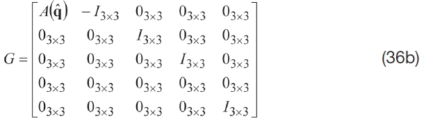
The new augmented matrix Qaug corresponding to the new process noise vector defined in Eq. (35b) is given by
The state transition matrix for the error covariance can be computed numerically by van Loan’s method (Brown and Hwang, 1997) as
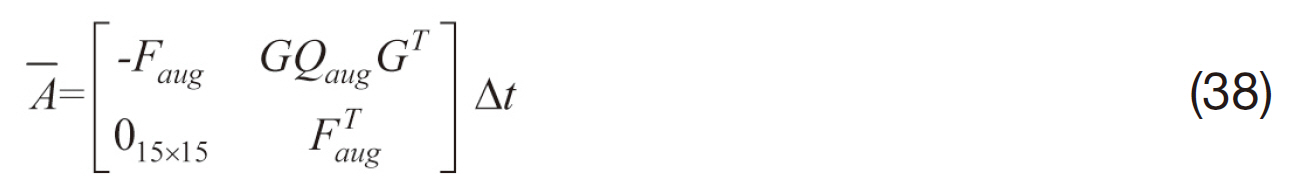
The matrix exponential of Eq. (38) is computed as
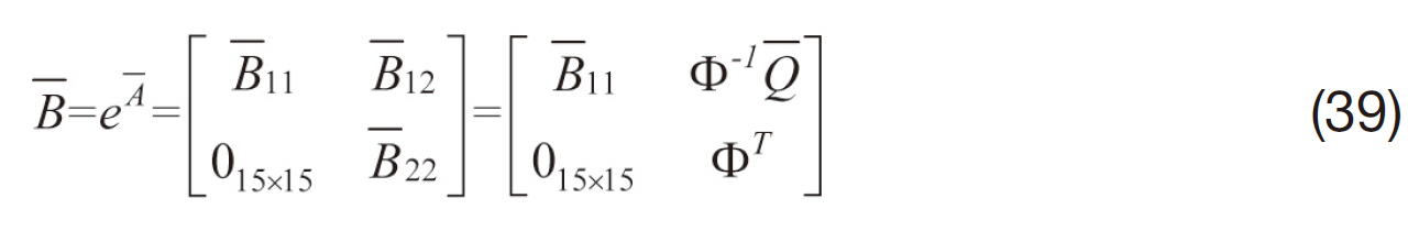
where Φ is the state transition matrix of Faug and ? is the discrete-time covariance matrix. The state transition matrix and discrete-time process noise covariance are then given by


The measurement sensitivity matrix (Kim et al., 2007) is given by
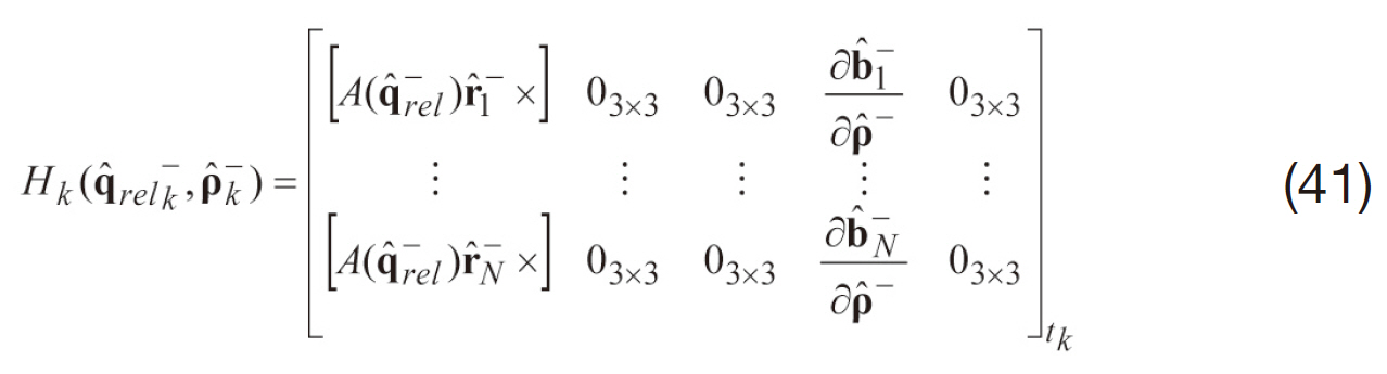
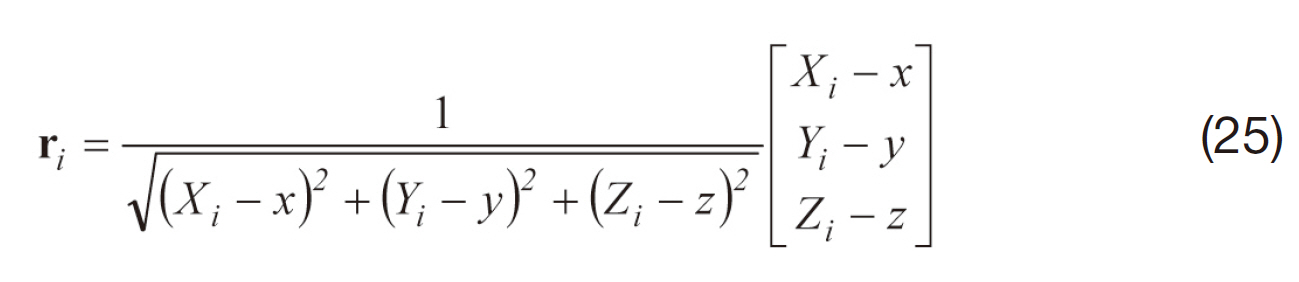
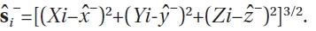
where ?i? is given by Eq. (25) evaluated at ρ??=[x?? y?? z??]T and the partial matrix ?b ?i?/ ?ρ?? is given by
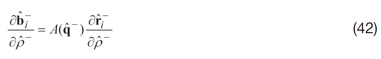
where
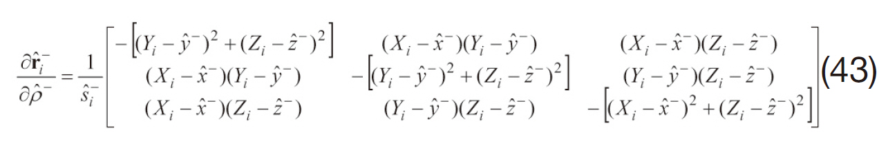
with
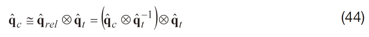
The estimated relative quaternion q?rel was then used to compute the absolute chaser quaternion by multiplying the known target quaternions by the target onboard navigation, namely
Optimal control techniques were used to provide translational and rotational maneuvering algorithms. The state-dependent Riccati equation (SDRE) (Cloutier, 1997; Stansbery and Cloutier, 2000) tracking controller designed for use with nonlinear relative dynamics was used to determine the required control forces for translational maneuvering. A LQG-type controller was derived for use in rotational maneuvering. By using thrusters for translational and rotational control, both can be uncoupled to a high degree of accuracy. However, unwanted thruster-induced torque was considered as a disturbance in the attitude controller. The two controllers were designed independently and executed on-board simultaneously.
7.1 SDRE tracking formulation for translational motion
An integrative approach combining a SDRE control and an EKF filter is introduced. The autonomous, infinite horizon, nonlinear problem for minimizing the performance index is considered.
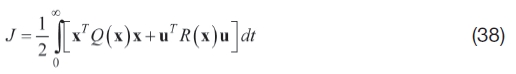
with respect to the state x and control u, subject to the nonlinear differential constraints:

where Q(x)≥0 and R(x)>0 for all x. The SDRE control method provided an approximate nonlinear feedback solution of the above problem. The SDRE design technique consisted of the following steps. First, the direct parameter method is used to bring the nonlinear equation into statedependent coefficients (SDC) form, which is a linear-like structure.

To obtain a valid solution of the SDRE, the pair {A(x), B(x)}has to be pointwise stabilizable in the linear sense so that for all x in the domain of interest a feasible (i.e., positive definite) solution may be obtained. Second, the SDRE is solved.

where, P(x) is state dependent, positive definite for x≠0. Third, the nonlinear feedback controller equation is constructed.

To perform command following, the SDRE controller can be implemented as a servomechanism, similar to that of an LQR servomechanism. The control state x is desired to track the reference commands xr(t). The modified SDRE servo controller is then given by

The estimated state with satisfied accuracy helped the SDRE controller track the reference state better, especially in the external disturbances and plant uncertainties. Thus, the EKF filter was combined with the SDRE feedback control law in Eq. (43) to replace the control state, x(t) by the estimated state, x?(t). Consequently, the nonlinear feedback controller equation is reconstructed.

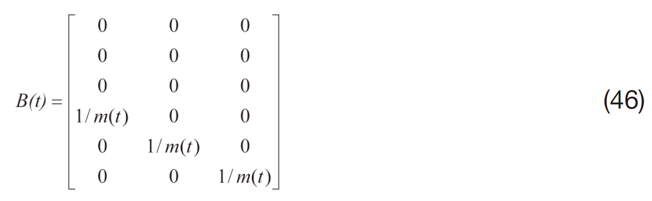
The spacecraft translational maneuvering was accomplished through the use of control force Fs∈R3. The nonlinear equations of the spacecraft dynamics in Eq. (5) are written in state-space form in the form of Eq. (39) to give
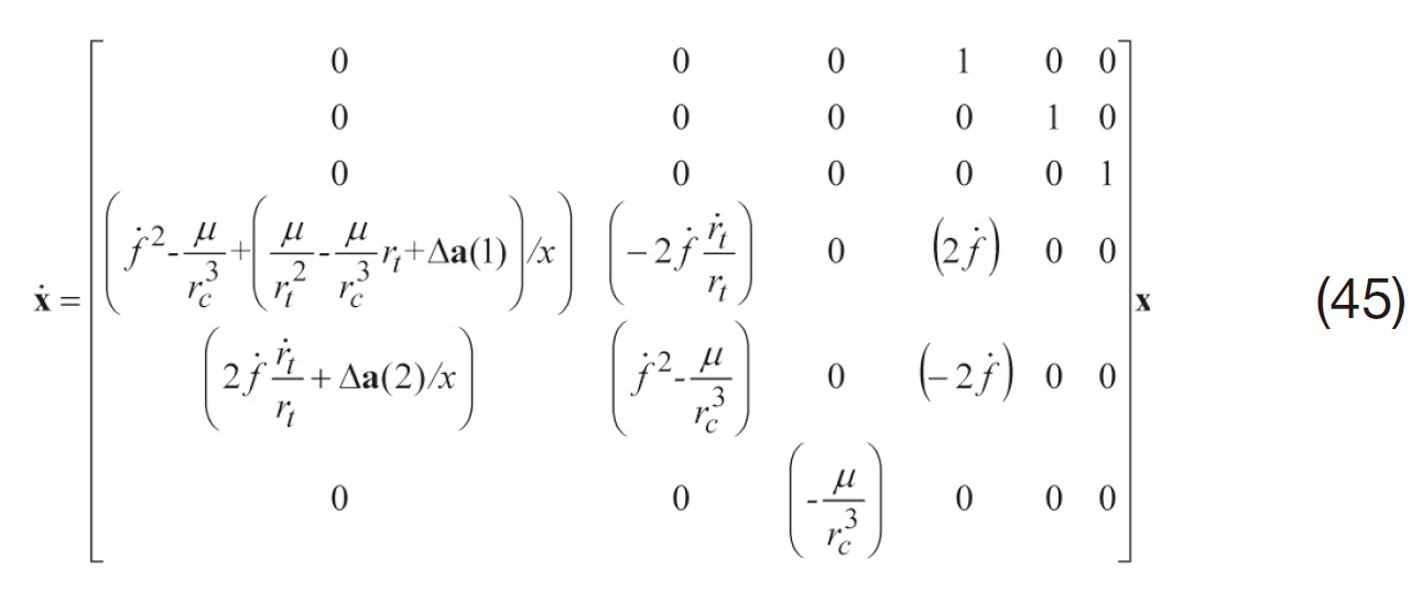
where the denominator x must not be allowed to be zero in order to avoid a singularity. The control distribution matrix, B(t) is
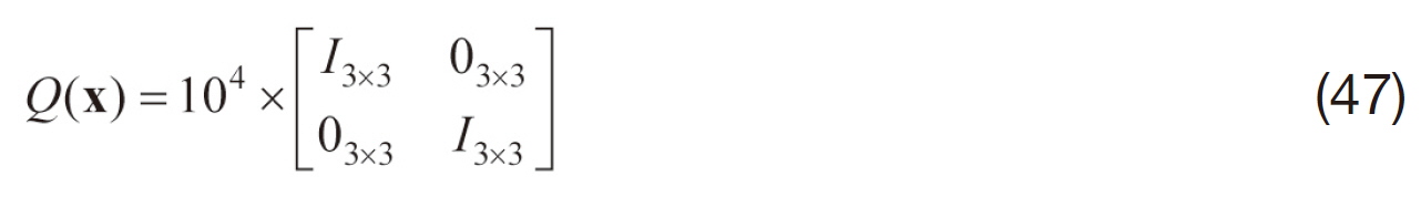
The state weight matrix for the performance index in Eq. (38) is given by
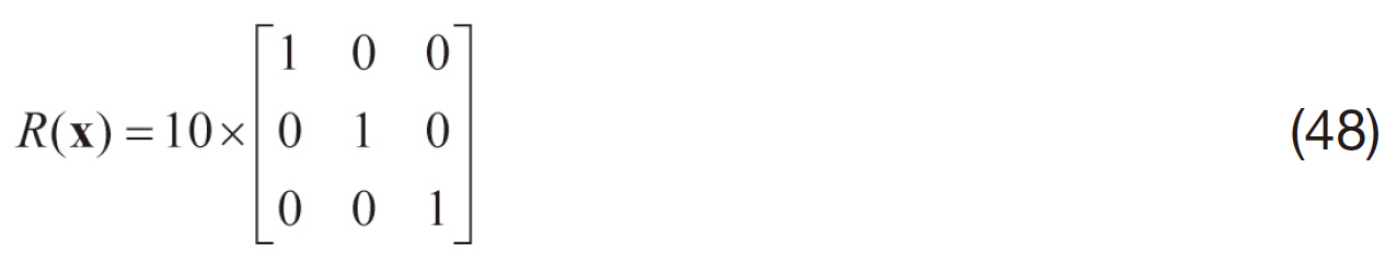
The control weight matrix in Eq. (38) is given by
The weight matrices used at the initial time were adjusted at steady state conditions in order to reduce the steady state tracking error. This readjustment was performed after the state estimation was stabilized to provide precise accuracy.
7.2 LQG-type control for translational maneuvering
The SDRE controller incorporated the EKF filter for relative position and velocity estimation, and guidance for the reference state. The SDRE control was then transformed into an LQG- type control (Brown et al., 1997). GNC functions were integrated into a feedback closed-loop system. This system became a key component of the integrated GNC system where the controlled state x(t) was replaced by the estimated state x?(t) and K(x)xr(t) was the feed-forward term. For this replacement to be valid, the separation principle must be met. Since the SDRE controller had a linear-like structure, and was controllable and observable, it met the condition for the separation principle, validating the design for the LQG-type controller.
7.3 LQG-based control for rotational maneuvering
Certain properties of quaternions provide linearization of the error dynamics formulation. Paielli and Bach (1993) presented linear quadratic regulator (LQR) approach with linearized dynamics using an optimal control design with linearized closed-loop error dynamics for tracking a desired quaternion. This study adopted this linearized equation to take advantage of the simplified equation of motion used to determine the precise attitude control. The control law formulation using LQR was combined with an EKF filter for attitude control, which led to the same LQG-type controller that was used for controlling the translational maneuvering. The chaser body-fixed frame must coincide with the target body-fixed frame at the moment of docking. The goal was to drive the state to zero while minimizing control energy expended. The regulator problem was then formulated with the performance index.
where x(t) is the attitude quaternion. The kinematic equation for the desired or reference quaternion qd is given by
where ωd is the desired angular velocity vector and qd is assumed to be provided by the target onboard navigation system. The error quaternion is defined as
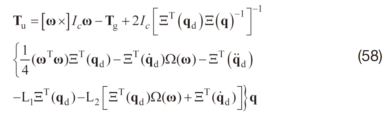
Similar to the way in which the weight matrices were adjusted at steady state for translational control, they were also readjusted at steady state to reduce the attitude tracking error. The algebraic Riccati equation was solved to compute a constant gain matrix, and it was then required to find a control torque input Tu in Eq. (13) that satisfied the linear form given in Eq. (53). Through differentiation and substitution, a control torque input Tu (Crassidis and Junkins, 2004) is derived as
For precision attitude control with robustness to the moment of inertia and external disturbances, accurate attitude sensors were specified and the EKF was combined with LQR control. The EKF estimated the gyro biases along all three axes and the quaternions of the chaser spacecraft. The sensors used here included three axis gyros and star trackers whose output was the attitude quaternion referenced to J2000 inertial coordinates. The noise parameters for the gyro measurements were the same as given in the previous section. A combined quaternion from two star trackers was used as the measurement. To generate synthetic measurements, the following model (Brown and Hwang, 1997) is used:
where, q is the truth, and v is the measurement noise, which is assumed to be a zero-mean Gaussian noise process with covariance of 0.001I3×3deg2. The quaternion measurement was then normalized to satisfy the unity quaternion constraint. An error quaternion between the measured quaternion and the estimated quaternion was used for measurement in the filter, computed using
where qe is the estimated quaternion of the chaser spacecraft. Although parameter uncertainties existed, such as the moment of inertia or external disturbances, the quantity qe can still be precisely estimated with high precision sensors. The benefit of robustness in control toque was then achieved by providing the estimated quaternion that coped with such factors
8. Numerical Results and Analysis
The proposed integrated system is illustrated using the modified ATV approach strategy described previously. The initial chaser (ATV) position was [0.2 -3500 0.1] m with respect to the docking port in the CW frame. The target moment of inertia (Fehse, 2003) and the chaser moment of matrix (Nagata et al., 2001) are given as
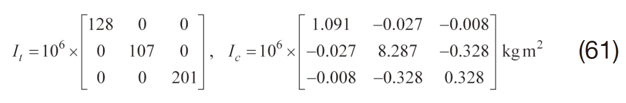
The initial mass of the chaser (Fehse, 2003) in this scenario was assumed as the ATV’s launch mass of 19,600 kg, and was time varying as the propellant was consumed. The propellant consumption was assumed to be known. The simulation was conducted in a predefined step-by-by step manner and continued to run until the docking port of the target was impacted, assumed to have coordinates [-1.02 -20.0 0.0] m in the CW frame. The initial relative position and velocity of the chaser in the CW frame (in units of meters and meter per second) are given by

The initial attitude of the chaser was rotated by 1 degree of roll, 5 degrees pitch and 1 degree of yaw with respect to the CW frame of the target. These values corresponded to initial roll, pitch, and yaw angles of the chaser with respect the inertial frame as φ=175.21, θ=?7.02 and ψ=56.89degress in a body 3-2-1 sequence. The corresponding chaser quaternion is then given by

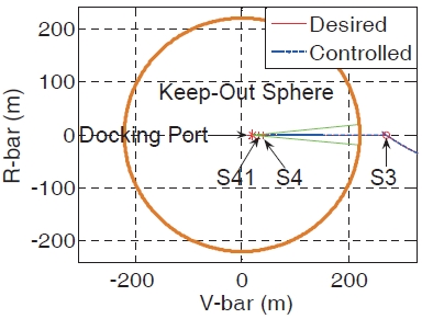
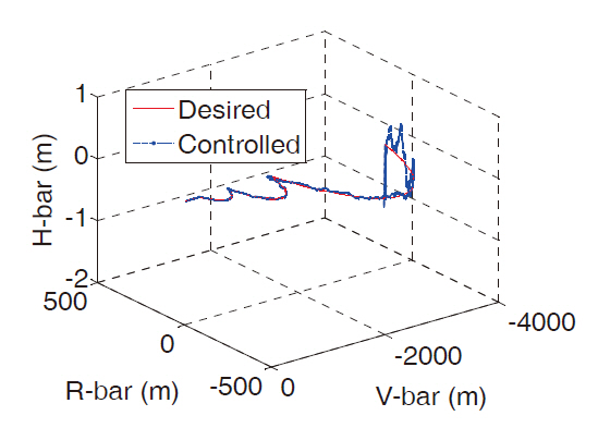
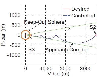
The simulation was performed for 91 minutes at a 0.1 second step size. The spectral densities of the process noise components to be added to the right-hand side of Eq. (5) which were to be adopted as the truth model were each given by 10?7m/(s s ). Figure 3a shows the overall approach trajectory from S2 to the target docking port, successfully tracking the desired nominal path including the V-bar hops. The S2 location was 3.5 km away from the target docking port, where, in general, a distance between 1 and 3 km was considered close-range rendezvous. Ensuring that the chaser entered the approach corridor and passed through it without crossing the keep-out sphere for proper alignment for the final straight line approach was critical. The approach
trajectory in Fig.3b shows that it safely entered within ±5 degrees of the approach corridor after stationkeeping at S3.
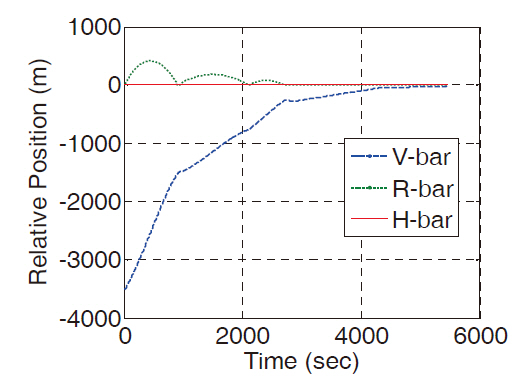
The final straight line approach was then executed with the navigation system switching from the RELAVIS scanning system to the VISNAV system at S4 to provide more accurate navigation and attitude estimation. The entire proximity operations trajectory is shown in three dimensional space in Fig. 4 Figure 5 shows the relative position history.
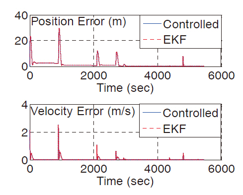
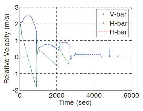
The relative position tracking error and approach velocity histories, shown in Figs. 6 and 7 were used to ensure that
the docking conditions (shown in Table 2) were met. After the chaser vehicle executed the final stationkeeping at S4, its position tracking error, which was less than 0.07 m, was maintained to the docking port and satisfied the lateral misalignment condition (less than 0.1 m). The relative velocity history along each direction, shown in Fig. 7,was less than 0.07 m/s and satisfied the longitudinal closing and lateral velocity conditions during the straight line approach.
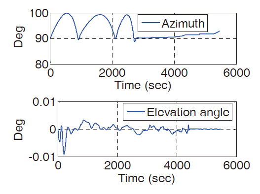
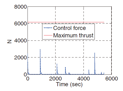
A nominal docking orientation with the target along the positive V-bar direction corresponded to an azimuth angle of 90 degrees. However, the docking port geometry was not aligned with the target center of mass, the target center of mass, the docking port location was not located precisely along the V-bar direction. The actual azimuth angle was 93 degrees. Figure 8 shows that the azimuth angle variation was less than 10 degrees and the elevation angle variation was near zero since the approach trajectory occurred within a plane. Whenever the GNC system reinitialized at each assigned point of the subsequent phase, the control forces exhibited large impulsive reactions as shown in Fig. .9 The weight matrices were readjusted at steady state to reduce the tracking error without causing thruster saturation. Of course, it was critical that the SDRE controller command realizable
control forces to the actuator (RCS) without exceeding the maximum available thrust.
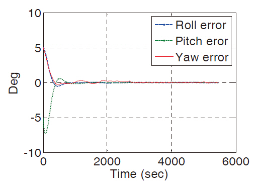
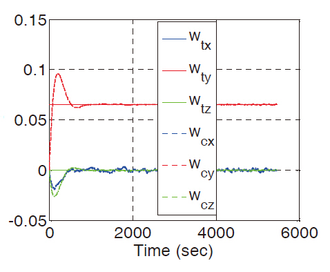
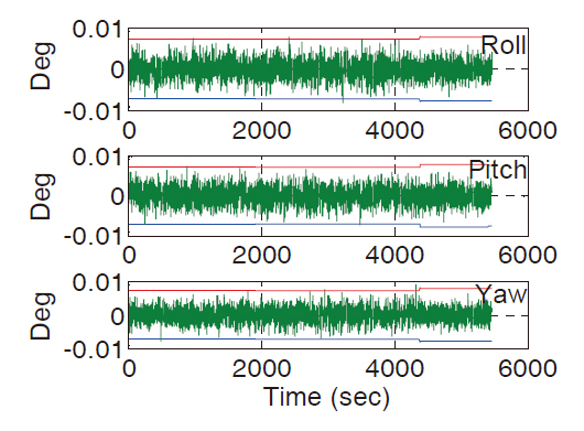
As propellant was consumed, the mass and moment of inertia of the chaser varied. An assumption of this study was that the locations of all RCS thrusters were known, and that the propellant mass consumption resulting from application of the control forces and torques can be readily computed. The robustness of the attitude controller was evaluated in the presence of uncertainties in the moments of inertia. The uncertainty was quantified by adding 30 percent of the moment of inertia to the initial value. Additionally, random external disturbances, which were not modeled in the controller, were included as modeled in the Euler rotational equation of motion in Eq. (13). Using the initial conditions given in Eq. (63), the chaser successfully performed the axis alignment with respect to the target. The weight matrices were adjusted in the attitude controller to reduce the attitude tracking error. Figure 10 shows the Euler angle error history between the target and the chaser. After the readjustment of the weight matrices, the chaser achieved attitude errors of less than 0.1 degree at the terminal time. Figure 11 shows the target angular rate and the chaser successfully tracks the target’s attitude rate for 1,000 seconds. The chaser pitch
[Table 2.] Conditions for successful docking (3σ)(Pinard et al. 2007)
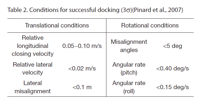
Conditions for successful docking (3σ)(Pinard et al. 2007)
rotation rate approached the mean motion rate of the target as the attitude alignment was achieved. Figures 10 and 11 demonstrate that the important rotational conditions listed in Table 2 were met.
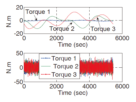
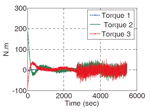
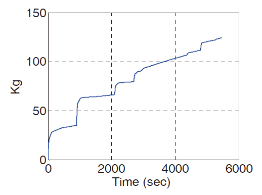
The upper graph in Fig. 12 shows the gravity-gradient torque history and the lower graph shows the random external disturbance torque history. Figure 13 shows the control torque history under the uncertainty in the moment of inertia, the gravity-gradient torque, and the random external disturbance torque, which exhibits some random behavior caused by the external disturbance torque, demonstrating the overall robustness of the controller. Figure 14 shows the propellant consumption by the application of control forces and control torques. Figure 15 shows the absolute attitude estimation and respective 3σ bounds by the RELAVIS scanning system from S2 to S4.
An integrated system composed of guidance, navigation and control for autonomous proximity operations and docking was developed and evaluated. The integrated system performed each phase in a predefined step-by-step manner autonomously. The integrated system integrated the independent guidance, navigation and control functions in the form of linear quadratic Gaussian-type control. The position tacking controller was developed by employing state-dependent Ricatti equation control without increasing the state dimension. The attitude tracking controller was developed by employing the linear quadratic regulator control. A variety of navigation systems were used in each phase to provide more efficient state estimation. The weight matrices in the controllers were readjusted autonomously along the filter convergence to achieve the better tracking. A six degree-of freedom simulation demonstrated the integrated system can execute several translational and rotational maneuvers that satisfy docking conditions.