An extended scalar adaptive filter for guided missiles using a global positioning system receiver is presented. A conventional scalar adaptive filter is adequate filter for eliminating sudden abnormal jumping measurements. However, if missile or vehicle velocities have variation, the conventional filter cannot eliminate abnormal measurements. The proposed filter utilizes an acceleration term, which is an improvement not used in previous conventional scalar adaptive filters. The proposed filter continuously estimates noise measurement variance, velocity error variance and acceleration error variance. For estimating the three variances, an innovation method was used in combination with the least square method for the three variances. Results from the simulations indicated that the proposed filter exhibited better position accuracy than the conventional scalar adaptive filter.
Since World War II, guided missiles have grown into an immense field of research and development for modern warfare. Presently, guided missiles use global positioning systems (GPS) to locate and obtain a position. However, several disturbances can affect GPS signals. As a result, abnormal or unintentional missile positions may be administered to a missile by the GPS. Thus, adequate filtering algorithms are necessary for eliminating an abnormal estimated position. Conventional scalar adaptive filters are adequate filter algorithms that eliminate strange signals (Cho et al., 2002; Lee et al., 2001; Maybeck, 1979; Mehra, 1972; Salychev, 1998). In general, the conventional filter assumes that a missile travels at a constant velocity. However, missile velocities tend to vary during practical applications. If a missile possesses an acceleration variance, a conventional filter cannot guarantee satisfactory filter performance.
Outlier detection methods based on graphs, densities and distances can be employed for eliminating abnormal signals. Graph-based methods were proposed by Hautamaki et al. (2004) In Hautamaki’s method, outlier detection using indegree number (ODIN) algorithms that utilizes k-nearest neighbor (kNN) graph. A kNN graph is a weighted and directed graph in which every vertex represents a single vector, and the edges correspond to pointers to neighboring vectors. Density-based methods originated from statistical analyses. In density-based methods, an object is considered an outlier if it greatly deviates from the underlying distribution. Examining the behavior of high dimensional data in a lower dimensional subspace is the preferred procedure for density-based methods. Effectively detecting outliers using full dimensional measurements would be difficult because of the averaging behavior of noisy and irrelevant dimensions. Thus, Aggarwal and Yu (2001) defines outliers by identifying projections in the data that possess annormally low densities. Abnormally low dimensional projections are defined as projections in which the density of the data is exceptionally different from the average density.
In distance-based methods, an outlier is defined as an object that is at least some distance away from some percentage of the objects in the dataset. The problem is then determining an appropriate distance and percentage such that the outliers would be correctly detected without allowing too many false detections (Hautamaki et al., 2004; Ramaswamy et al., 2000). However, outlier detection methods do not properly fit the needs of missile guidance because these methods possess heavy calculation loads.
Thus, we proposed an extended scalar adaptive filter. The proposed filter continuously estimates noise measurement variance, velocity error variance and acceleration error variance. For estimating three variances, an innovation method was used in combination with the least squares method for the three variances. Results from the simulations indicated that the proposed filter exhibited better position accuracy than the conventional scalar adaptive filter.
The conventional scalar adaptive filter state is a simple one dimensional quantity. This filter easily eliminates abnormal peak errors by using an adaptive method, which continuously estimates measurement errors and velocity error variance. When the measurement jumps to an abnormal point, the measurement error will increase and the innovation increases. The filter gain decreases. Therefore, the filter will not react to unnecessary abnormal measurement jumps.
The discrete model is represented by

where Xk-1 is the state, Vk-1 is the derivative of the state, T is the sampling time and ek is the measurement noise.
The conventional scalar adaptive filter algorithm is described in Eq. (2). Adaptive methods encompass the innovations method and the least square method. If adaptive methods are not applied to the filter, the filter will use two fixed values: the measurement noise variance Rk and the velocity error variance qk. In this case, the filter can only eliminate minimal jump errors (Cho et al., 2002; Lee et al., 2001; Maybeck, 1979; Mehra, 1972; Salychev, 1998).
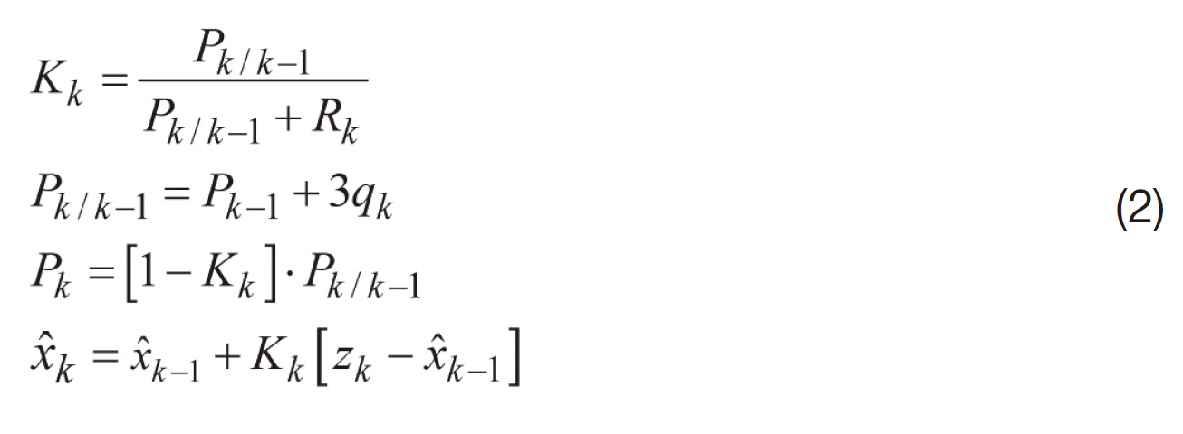
where, x?k is the estimate of the state, Kk is the filter gain and Pk is the error variance.
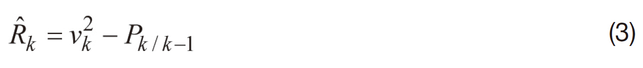
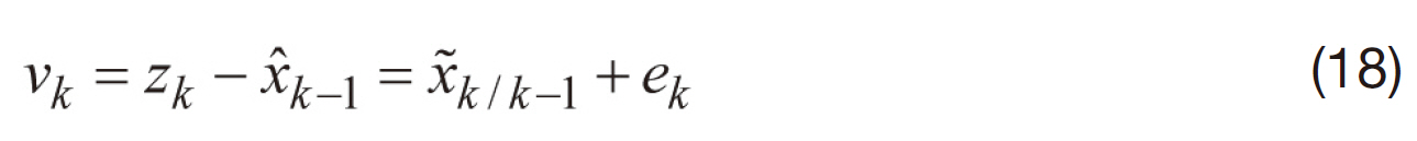
To make the filter more adaptive, we Rk and qk should be changed in each step. By introducing the innovation sequence vk=zk?x?k?1, the measurement noise variance can be estimated as Cho et al. (2002), Lee et al. (2001), Maybeck (1979), Mehra (1972), and Salychev (1998)
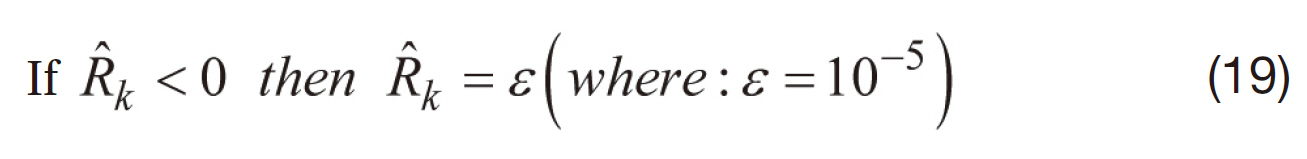
During the calculation procedure the estimate of Rk may become negative. In order to overcome this obstacle, a normalization procedure must be introduced. To incorporate this procedure, one more parameter qk is necessary. In general, qk is related to missile dynamic and the process noise model. In contrast, qk represents the velocity error variance in the conventional scalar adaptive algorithm. The least square method must be used to estimate a suitable value for qk. An estimation procedure can be used to calculate qk to ultimately obtain a universal algorithm.
Let us define
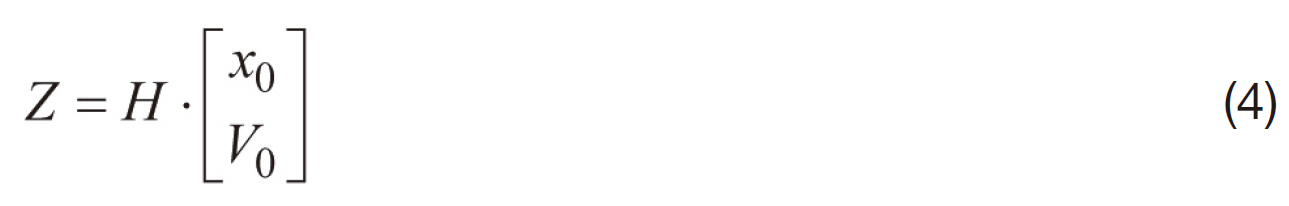
where,
T refers to the sampling time; x0, V0 represents the initial values of each parameter; N is the number of measurements for least square method.
The least square estimation for Eq. (4) can be introduced as
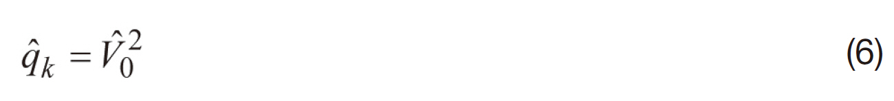
Therefore, the estimation of qk is obtained by
Using above the conventional scalar adaptive filter algorithm, we can easily eliminate sudden strange jump signals. The accurate performance of the conventional filter, however, cannot be guaranteed, especially when the speed of the missile exhibits sudden changes.
3. Extended Scalar Adaptive Filter
3.1 Filter algorithm extension
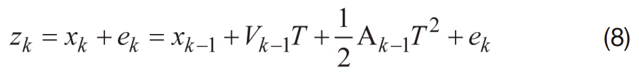
In order to overcome the disadvantages of the conventional scalar adaptive filter, an acceleration term was taken into consideration for the extended scalar adaptive filter. Therefore, Eq. (1) can be rewritten as
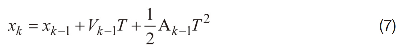
where Ak is the acceleration. The measurement equation can be modified as
In order to calculate the covariance of a state variable, the difference between true state and estimated state was first calculated, as follows
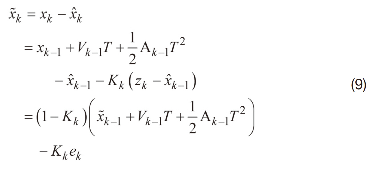
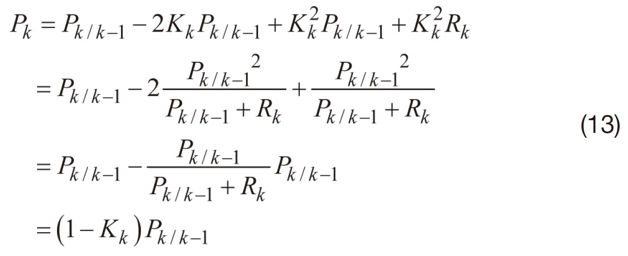
Then, the error covariance Pk was constructed
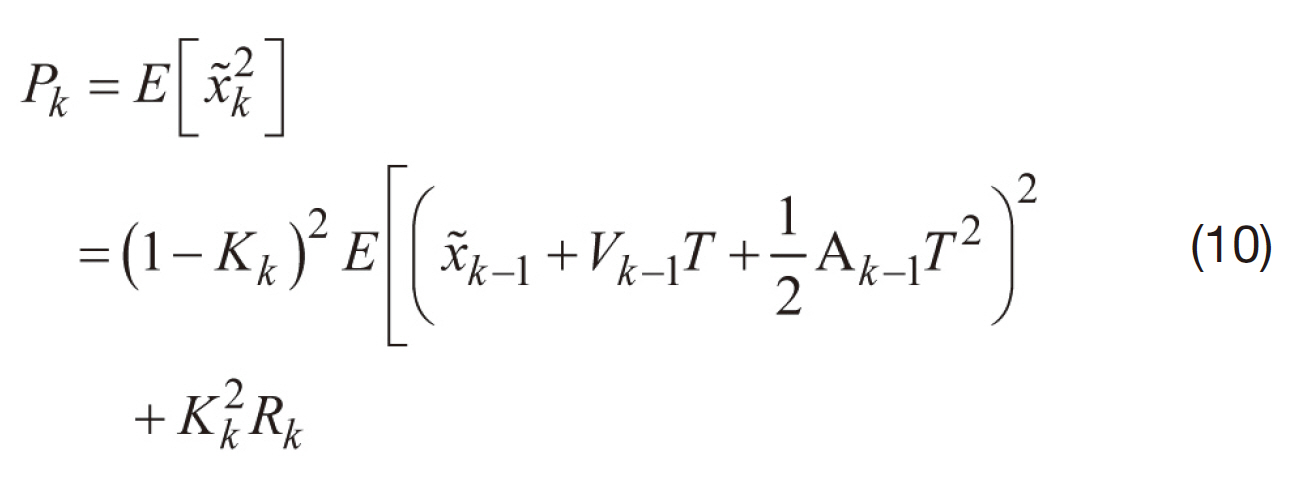
where Rk=E[e2k]. Defining
obtaining the following
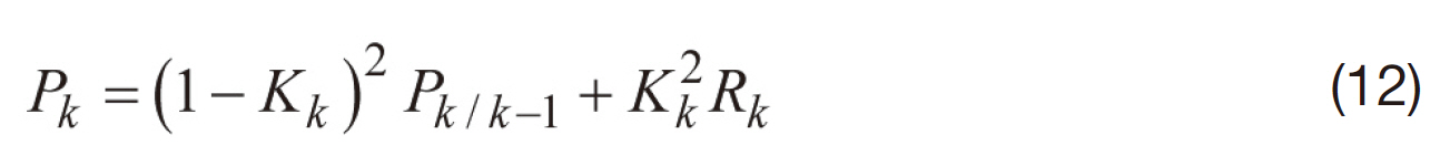
Using Eq. (12), Kkwas calculated in order to derive the minimized value Pk: Kk=Pk/k?1/Pk/k?1+Rk. After substituting Kk into Eq. (12), the following was achieved
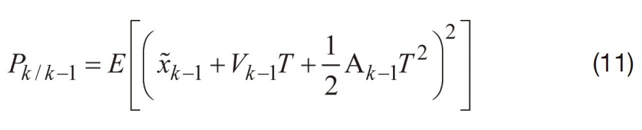
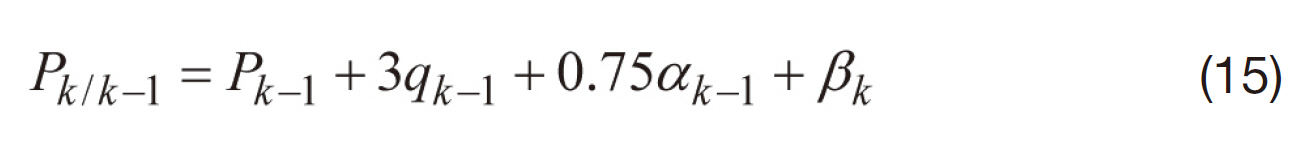
In order to complete the extended scalar filter algorithm, Pk/k?1 should be calculated as
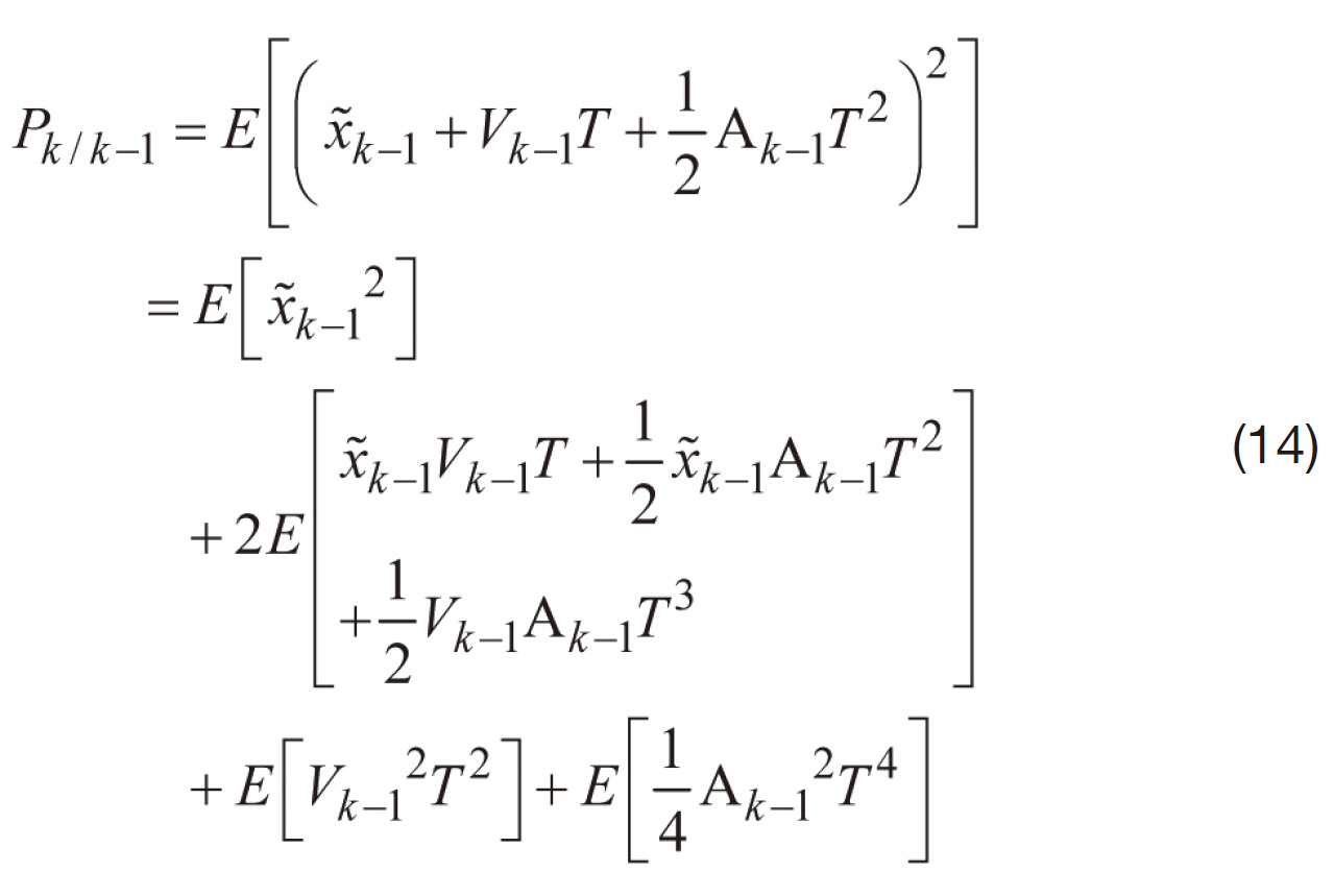
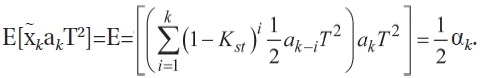
To obtain Pk/k?1, the steady state filter gain was needed. This gain can be retrieved through a simulation or analysis of the sample signal. For this study, the gain was determined to be 0.5, and the missile was assumed to travel with a constant acceleration during a very short sampling period. Defining αk=E[Ak2T4], βk=E[Vk?1Ak?1T3] and qk=E[Vk2]T2, we calculated
Similar to the conventional filter derivation method, we obtained
For estimating Rk, the innovation method was used. This procedure is a meaningful aspect of the extended scalar adaptive filter, facilitating the filter to eliminate sudden abnormal jumps in measurements. When a measurement jumps to an unknown point, innovation will increase. Thus, the filter will not react to abnormal measurement errors.
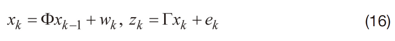
Generally, mathematical representation of filter model can be introduced (Brown and Hwang, 1997)
Innovation sequence is introduced as follows:
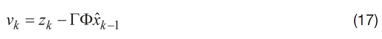
In the scalar filter case, Γ and Φ are 1. Eq. (17) can be rewritten as
R?k can be obtained by using the same method as in the conventional filter. Also, we applied the following condition in order to prevent numerical errors.
The velocity error variance as well as the acceleration error variance must be estimated. These parameters are related to the estimate of the noise measurement variance. Thus, these two parameters must be continuously estimated. From Eq.(7), we can derive
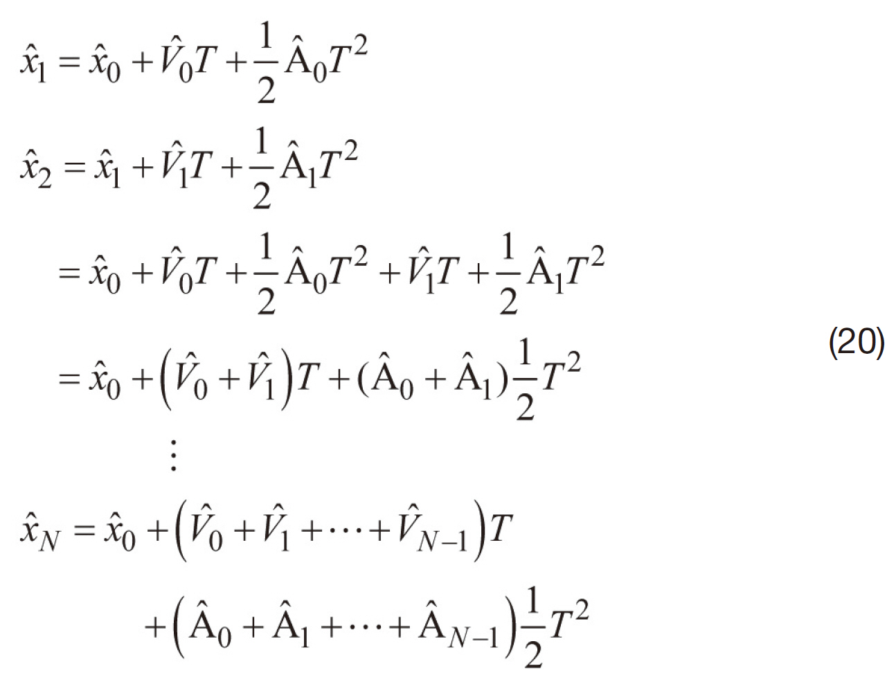
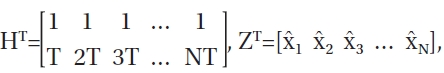
where N is the number of measurements, which must be used for the least square method. The filter cannot estimate a state value when N is too large or small. This parameter is not a fixed value and changes depending on the system. If the acceleration is same for sufficiently short sampling time interval, Eq. (20) can be expressed in the matrix form,
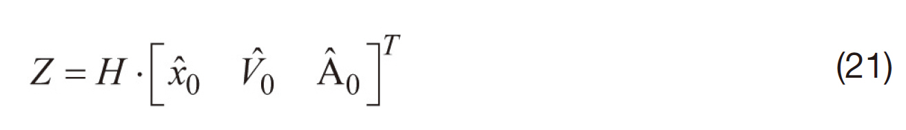
where,
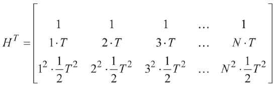
ZT=[x?1 x?2 x?3 … x?N].
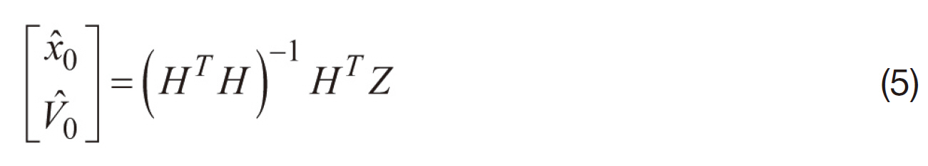
To accurately estimate qk and αk, the least square method was introduced. With previous N samples, the least square solution of Eq. (21) can be obtained as follows:
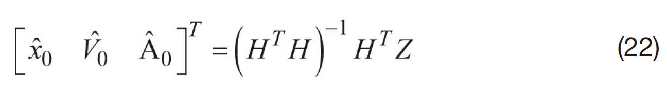
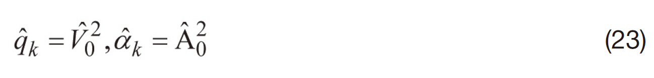
Using the above relation, the velocity and acceleration error variances were obtained as
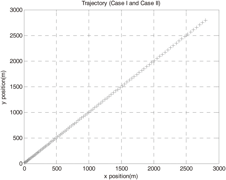
Three different simulations were conducted in order to verify the extended scalar adaptive filter’s performance. Simulation cases I and II were conducted under a constant acceleration condition. Simulation case III incorporated the surface-to-surface missile (SSM) trajectory. The sampling rate was 100 Hz for the SSM trajectory. Six measurements were used to estimate qk and αk within the proposed filter in each step. Figure 1 shows case I and II trajectory for SSM launch part.
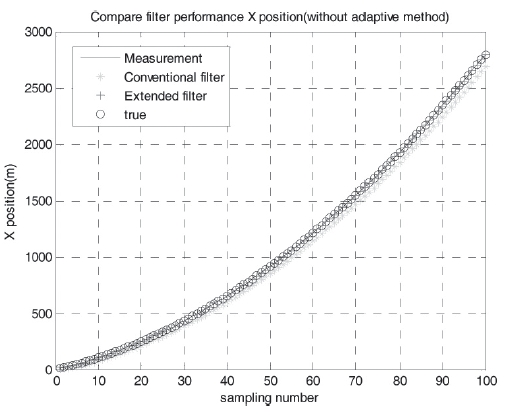
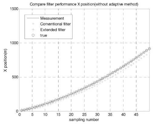
Figure 2 shows the constant acceleration case without adaptive methods. There are no sudden changes in measurements. Under ideal circumstances, all filters must estimate accurate positions. However, the conventional filter was unable to accurately estimate missile position. Furthermore, the position error of conventional filter grew as time passed. The position of the conventional filter’s root mean square (RMS) error was 68.6 m, but that of proposed filter was only 2.9 m.
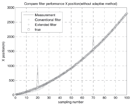
Figure 3 describes case II results. Case II had the same trajectory as case I, but case II exhibited two abnormal jump measurements. In case II, the conventional filter’s
convergence speed was slower than that of the proposed filter. In order to estimate the position based on the proposed filter, only 6 measurements were necessary, which were comparable to 9 samples in the conventional filter. When only 6 measurements were applied to the conventional filter, the filter did not perfectly estimate missile position.If an abnormal jump error occurred within 9 samples, the conventional filter did not perfectly eliminate the abnormal measurement. In other words, the conventional filter required more information than the proposed filter. Thus the proposed filter more accurately eliminated abnormal measurements using less sampling data than the conventional filter. Additionally, the proposed filter exhibited a faster convergence speed than the conventional filter. For case II, the proposed filter’s RMS error position was 3.4 m while the conventional filter was 29.7 m.
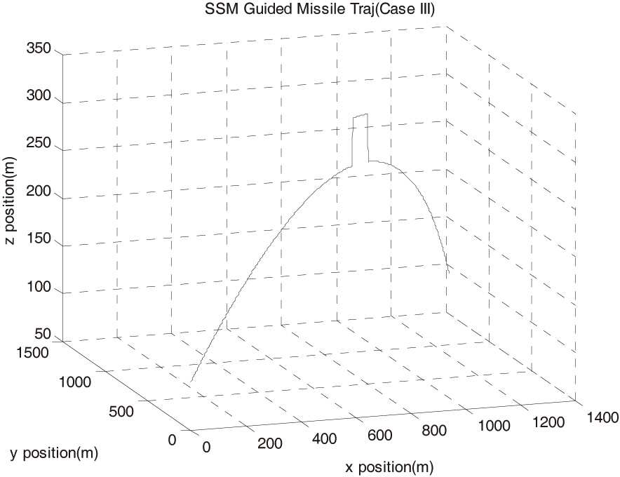
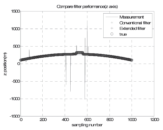
Figure 4 shows case III SSM trajectory. This missile used GPS for obtaining missile position. We assumed the missile used avoidance movement between 500 and 565 samples in order to defend from defensive missiles, such as an antiballistic missile. In particular, the acceleration of the missile rapidly changed rapidly during the avoidance movement period.
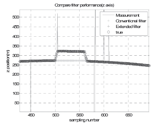
Figure 5 represents filter performances for the SSM case III. The conventional filter and the proposed filter both eliminated abnormal errors. However, the conventional filter did not offer suitable position solutions within the avoidance movement period. This is because the conventional filter failed to detect the avoidance period as an actual trajectory. In other words, the reaction of the conventional filter showed a much slower speed than that of the proposed filter. When the missile experienced velocity variations, the extended scalar adaptive filter was more proper than the conventional filter. In case III, the position of the RMS error of conventional
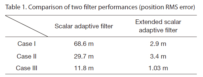
[Table 1.] Comparison of two filter performances (position RMS error)

Comparison of two filter performances (position RMS error)
filter was 11.8 m and the proposed filter was 1.03 m. Table 1 shows the result of filter performance comparison.
The conventional scalar adaptive filter is a suitable filter for eliminating abnormal jump signals. The conventional filter assumed that the vehicle moved at a constant velocity for a sufficiently short sampling time interval. Thus, the filter performance was limited by the above assumption. In particular, the vehicle exhibited a sudden variation in acceleration. In order to overcome this sudden change, the extended scalar adaptive filter was proposed. The filter algorithm was reformulated and was able to estimate one more adaptation parameter, the acceleration error variance. To verify the proposed filter’s performance, three different simulations were conducted. As a result, the position of the RMS error of the proposed filter decreased in comparison to the conventional scalar adaptive filter. In particular, the proposed filter reacted very quickly to sudden acceleration changes. Therefore, the proposed filter was a very adequate filter algorithm for eliminating sudden jump signals.