Formation flying, autonomous rendezvous and proximity operations typically require the high precision determination of relative attitude and position. The vision-based navigation (VISNAV) system can determine these types of information during the terminal phase of a rendezvous (Junkins et al.,1999). The VISNAV system has several advantages such as variable sensor size a different size sensors, wide sensor field of view, rapid image processing, relatively simple electronics, and minimal six-degree of freedom (DOF) data errors (2 mm in position estimates and 0.01o in attitude estimates at rendezvous) (Gunnam et al., 2002). Recently, space missions have relied on global positioning systems (GPS) that are integrated with other sensors including inertial navigation systems (INS), star trackers, and so on. A GPS-only navigation system may not be effective in space missions because it is subject to errors, integrity problems due to multipaths and other sources, or outage due to blockage, atmospheric ionization during re-entry and delta-v maneuvers (Gaylor and Lightsey, 2003). Although an integrated GPS/INS navigation system may meet the navigation requirements of all flight phases of a spacecraft in near-Earth orbit by system complementation, the VISNAV system only can meet the navigation requirement in the terminal phase of rendezvous without any limitations in GPS navigation. The sensor measurements used in this work are based on a VISNAV system which compromises an optical sensor of new kind combined with the specific flight sources (beacons) to achieve selective or “intelligent vision.” The sensor is made of a positioning sensing diode (PSD) placed in the focal plane of a wide angle lens (Junkins et al., 1999; Kim et al., 2007). A PSD-based sensor is mounted on the deputy vehicle, with structured-frequency light emitting diode (LED) beacons mounted on the chief vehicle. When the rectangular silicon of the PSD is illuminated by the energy from the beacon focused by the lens, and this illumination generates electrical currents in four directions. These currents can be processed with appropriate electronic equipment to estimate the energy centroid of an image (Kim et al., 2007). Intelligent vision uses the PSD to see only specific light sources, by modulating the frequency domain of the chief light and applying relatively simple analog signal processing (demodulation). A more detailed description of the VISNAV system can be found in Junkins et al. (1999) and Kim et al. (2007).

The extended Kalman filter (EKF) has been widely used in state estimation. The EKF is based on the approximation of the state distribution as a Gaussian random variable (GRV) which is propagated through first-order linearization of the nonlinear system. The EKF is a suboptimal filter because of the truncation of the higher-order terms to linearize a system. This truncation can cause large errors in the true posterior mean and the covariance of the transformed GRV, which may lead to suboptimal performance of estimation and sometimes divergence of the filter. The EKF may not be able to cope with realistic initial conditions, leading to filter divergence. Alternatives that can avoid the loss of higherorder terms are the unscented Kalman filter (UKF) and the particle filter. In this work, the UKF is applied to state estimation, because of its robustness under realistic initial conditions. The UKF is an extension of the traditional Kalman filter. It estimates nonlinear systems and performs the unscented transformation. The unscented transformation uses set of samples, or sigma points, that are determined from the a priori mean and covariance of the state. The sigma points completely capture the true mean and covariance of the GRV, and when propagates through a nonlinear system, they capture the posterior mean and covariance accurately to the third order of the Taylor series expansion for any nonlinearity (Lefferts et al., 1982). The ability of the UKF to estimate nonlinearities accurately makes it attractive for estimations of spacecraft relative attitudes and navigation, because of course, the state and observation models of spacecraft relative attitude estimation and navigation are inherently nonlinear.

In attitude representation, Euler angles, quaternions,classical Rodrigues parameters (or Gibbs vector), and modified Rodrigues parameters are typically used. Among these parameters, quaternions are attractive because there is no singularity and the kinematic equation is bilinear. As with the EKF, the direct application of the UKF with a quaternion parameterization of attitude yields a non-unit quaternion. The weighted sum of the quaternion samples in the UKF does not produce a unit quaternion space because the UKF is formulated in a vector space and the quaternion samples do not belong to a vector space but lie on a nonlinear manifold. To overcome this shortcoming, a quaternion multiplication, after neglecting higher-order terms in the error quaternion linearization, allows the four-component quaternion to be effectively replaced by a three-component error vector for the predicted covariance computation and quaternion update.

This guarantees that the quaternion unit normalization is maintained in the filter (Cheon and Kim, 2007; Crassidis and Markley, 2003; Shuster, 1993; VanDyke et al., 2006). The vision-based relative spacecraft attitude and position estimation based on the EKF under ideal initial conditions was researched by Kim et al. (2007). For example, Crassidis proposed using the UKF only for spacecraft absolute attitude estimation with realistic initial attitude and gyro bias measurements. Based on this previous research, this paper presents an extension of the UKF formulation to estimate the relative attitude, the relative position, and the relative velocity instead of the absolute attitude estimation only using the VISNAV sensor approach coupled with gyro measurements from each spacecraft. The necessary equations for relative attitude estimation between two spacecraft are derived. The gyro biases of the chief and deputy spacecraft are estimated. Like the standard EKF, the direct use of UKF with a quaternion parameterization of the attitude leads to a nonunit quaternion estimate. To overcome this complication, this study employs an alternative approach that uses a threecomponent attitude-error vector to present the quaternion error vector (Shuster, 1993). Several three-component representations are possible, including the Gibbs vector, which has a singularity at 180o, and the vector of modified Rodrigues parameters (MRPs), which has a singularity at 360° (Shuster, 1993). Since this approach uses only a threecomponent representation for the attitude errors, singularity is never encountered in practice. Updates are performed using quaternion multiplication, naturally maintaining the normalization constraint. The error-state vector derived in relative attitude estimation is appended to include information on the relative position and velocity, the radius and the radial rate of the chief, and the true anomaly and its rate. Thus, the objective of this paper is to propose a VISNAV system which estimates the relative attitude, relative position, and relative velocity between the chief and the deputy spacecraft using the UKF under realistic initial errorconditions.

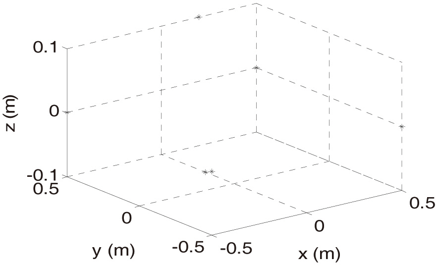
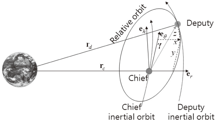
This section provides an overview of the model used to describe the relative position and attitude of a bounded out-of-orbit plane formation. From this formation, the relative equations of motion are then derived. Measurement equations are then derived for the VISNAV sensor, providing line-of-sight (LOS) vectors between the chief and the deputy spacecraft. This section presents the relative equations of motion and the methods to establish closed relative orbits. The chief inertial position vector is denoted as r_c, while that of the deputy inertial position vector is expressed as r_d. The relative position vector σ is expressed in Cartesian coordinate components as γ=(x, y, z)^T. The rotating reference frame used here is the common local-vertical-local horizontal (LVLH) Clohessy-Wiltshire (CW) frame. To derive the relative equations of motion expressed in CW Cartesian coordinates, the deputy position vector is written as r_d=r_c+ γ. This geometry is illustrated in Fig. 1.

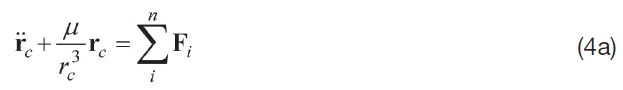
If the relative orbit coordinates (x, y, z) are small compared to the chief orbit radius rc, then the equations of motions are given by

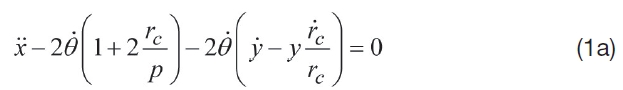
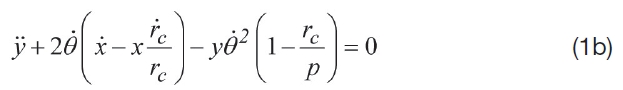
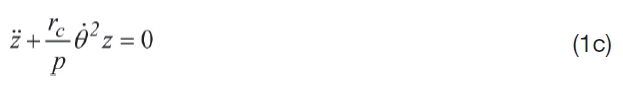
where p is semilatus rectum of the chief, r_c is the chief orbit radius and θ is true anomaly rate of the chief. These

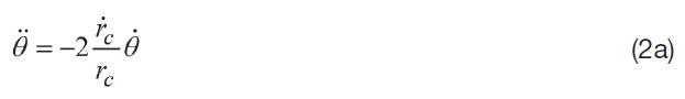
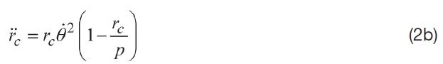
equations of motion are used as the system dynamic model in the filter. The true anomaly acceleration and chief orbitradius acceleration are given by

For generation of bounded relative motion to be used in the simulations, the initial condition at perigee is given by Schaub and Junkins (2003)

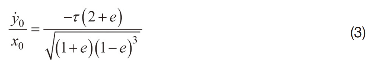
where τ and e are the mean motion and the eccentricity of the chief, respectively. The equations of motion hereassume that all perturbations are ignored. In reality, of course, there are many perturbations acting on the spacecraft. To validate the estimated states that yield the simulation results discussed below, the relative position and velocity are computed from two orbits expressed in Earth-centered inertial (ECI)reference coordinates and simulated by the high precision orbit propagator (HPOP) of satellite tool kit (STK) (Analytical Graphics Inc.). The true equations of motion, including the perturbations for the chief and deputy, are given by

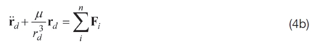
where μ is the gravitational coefficient and

the acceleration produced by the perturbations. In the geometry of the chief and deputy spacecrafts with the 3-1-3 rotation sequence illustrated in Fig. 2, the relative position and velocity vectors are derived from the position and velocity vectors using the inertial coordinates of the two spacecrafts. The Euler angles of the rotation sequence are as follows: Ω_c, which is the right ascension of the ascending node, i_c,which is the inclination angle, and θ_c which is the argument of latitude of the chief spacecraft. The position and velocity vectors of the deputy in the inertial coordinate are then expressed as

where C is the 3-1-3 rotation sequence, C=C₃(u_c)C₁(i_c)C₃(Ω_c), u_c, i_c and Ω_c is the argument of latitude, the inclination and the right ascension of the ascending node of the chaser,respectively. γ?is the relative velocity.

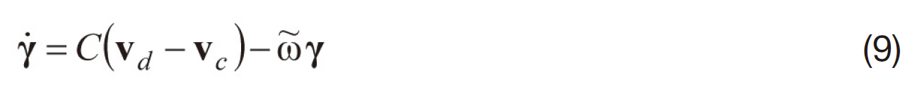
Also,

From Eqs. (5) and (6), the relative position and velocity vectors are determined as

This section briefly reviews the attitude kinematic equations using quaternions, the sensor models, and the UKF. In addition, a generalization of the Rodrigues parameter is briefly discussed. The quaternion is defined by q=[p^T q⁴]^T,with p=[q₁ q₂ q₃]^T=esin(？ /2) and q4=cos( ？/2), where e is the axis of rotation and ？ is the angle of rotation. Since a fourdimensional vector is used to describe three dimensions,the quaternion components cannot be independent of each other. The quaternion satisfies the normalization constraint q^Tq=1. The (relative) attitude matrix is related to the quaternion by

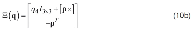
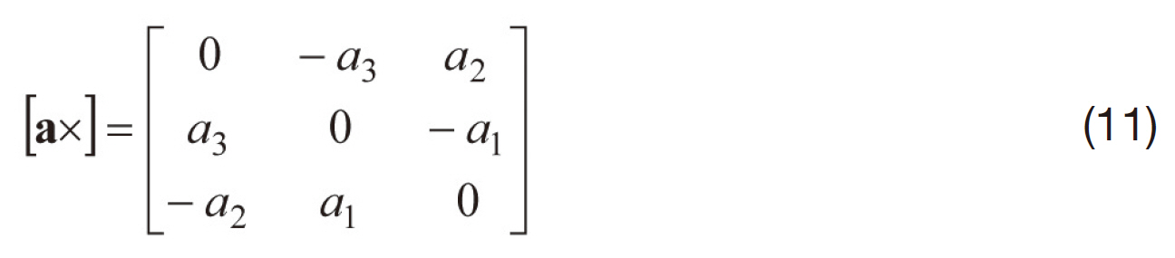
where I_3×3 is the 3×3 identity matrix and [ρ×] is a cross product matrix since a×b=[a×]b, with

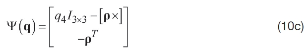
Quaternion multiplication permits successive rotations.Here, the convention of Lefferts et al. (1982) and Shuster(1993) is adopted, in which multiplies what? by the same order as the attitude matrix multiplication, A(q´)A(q)=A(q´？q). The composition of the quaternion is bilinear, with

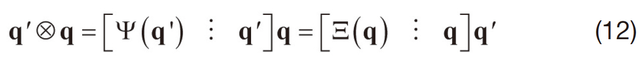
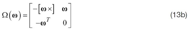
Also, the inverse quaternion is given by q^?1=[?p^T q₄]. Note that q´？q^?1=[0 0 0 1]^T, which is the identity quaternion. The quaternion kinematics equation is given by

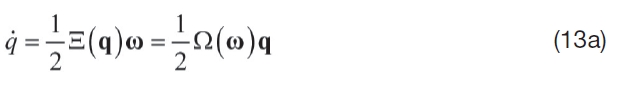
where

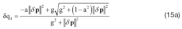
The local error-quaternion, denoted by δq=[δpT δq4] and defined in the UKF formulation, is represented using a vector of generalized Rodrigues parameters (Crassidis and Markley, 2003; Schaub and Junkins, 1996; Schaub and Junkins, 2003)

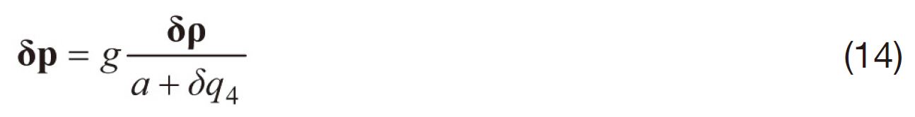
where α is a parameter from 0 to 1, and g is a scale factor. Note when a = 0 and g = 1, then Eq. (14) gives the Gibbs vector. Furthermore, with a = g = 1, then Eq. (15) gives the standard vector of MRPs. The effects of λ and the other parameter a to be explained later are demonstrated by simulations in Crassidis and Markley (2003). For small errors, the attitude portion of the covariance is closely related to the attitude estimation errors for any rotation sequence, given by a simple factor (VanDyke et al., 2006). For example, the Gibbs vector linearizes the half angles. g=2(a+1)is chosen so that ''δp'' is equal to ？ for small errors. The inverse transformation from''δp'' to δq is given by⁸

Vision-based discrete-time attitude measurements for a single sensor are given by Crassidis and Markley (2003), Gunnam et al. (2002), Junkins et al. (1999), and Kim et al.(2007)

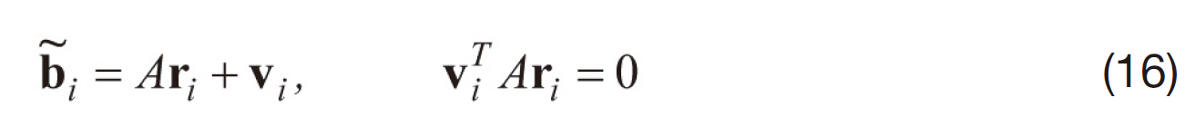
where b^~_i denotes the i^th observation and the sensor error v_i is characterized as being approximately Gaussian. This satisfies

where E{ } denotes expectation and I_3×3 denotes the 3×3 identity matrix. Multiple (N) vector measurements can be concatenated to form

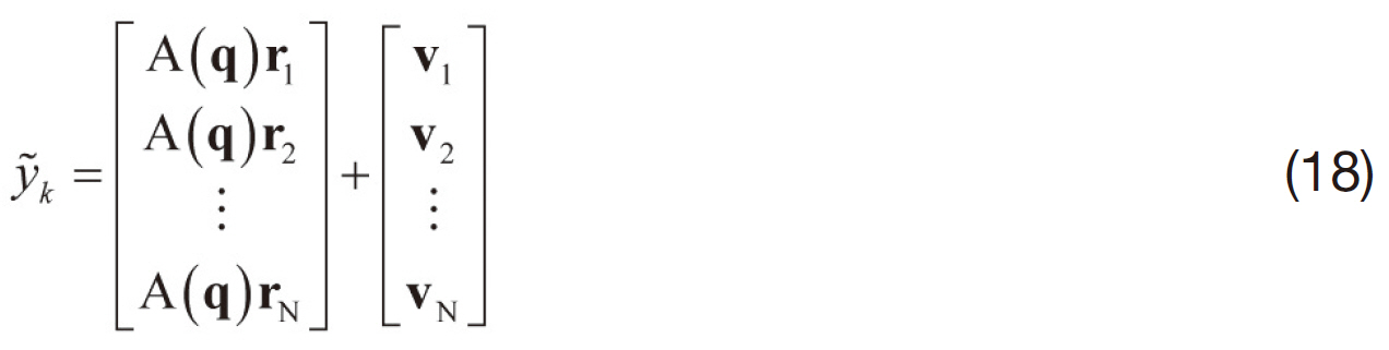
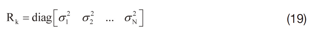
The advantage of using the model in Eq. (17b) is that the observation covariance in the UKF formulation can effectively be replaced by a nonsingular matrix given by σ_i ²I_3×3 (Schaub and Junkins, 1996; Shuster, 1990; Shuster and Oh, 1981). Hence, the observation covariance matrix used in the UKF from all available LOS vectors is given by

A common sensor that measures the angular rate is a rateintegrating gyroscope. For this sensor, a widely used model is given by Crassidis and Markley (2003) and Kim et al. (2007)

where ？ is the continuous-time measured angular rate, β is the drift rate, and η_v and η_u are independent zero-mean Gaussian white noise processes with

where δ(t-τ) is the Dirac delta function. In the standard EKF formulation, given a post-update estimate β⁺_k, the post-update angular velocity of the chief or deputy and its propagated gyro bias are

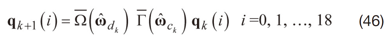
Given the post updates ？⁺_k and ？⁺_k, the discrete-time propagation of the relative equation of Eq. (13) is given by Kim et al. (2007)

With

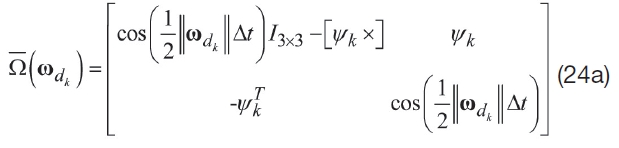
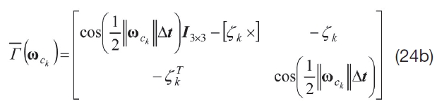
where

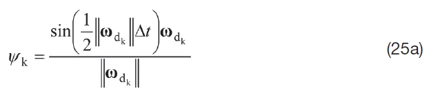
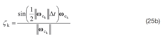
and Δt is the sampling interval. Note that the matrices ？^-(ωd_k) and Г^?(ωc_k) also commute. In this section, the UKF is also reviewed. Many difficulties in the EKF arise arises because of its linearization of a nonlinear system. To overcome the disadvantages of the EKF, the UKF uses an unscented transformation. Unlike the EKF, the UKF does not require Jacobian and Hessian computations. Rather, the UKF uses a minimal set of sigma points, deterministically chosen from the error covariance and propagated through the true nonlinear system to capture the posterior mean and covariance of the Gaussian random variable accurately for the third order Taylor series expansion for any nonlinearity (Cheng et al., 2006; Julier and Uhlmann, 2004; Wan and Van Der Merwe, 2000). (…to capture …covariance …accurately for the …) Consider the system model of discrete-time nonlinear equations

where x_k is the n×1 state vector and y_k is the m×1 observation vector. Note, that a continuous time model can always be expressed in the form of Eq. (26a) through an appropriate numerical integration scheme.7 The process noise vector w_k and observation noise vector v_k are assumed to be zeromean and white Gaussian noise, and the covariances of these vectors are given by Q_k and R_k , respectively. From the n×n covariance P_k , a set of (2n+1) sigma points X_k ∈²ⁿ⁺¹ can be generated by the columns of the matrices

The general formulation for the propagation equations begins with a set of sigma points with corresponding weights W_i, according to the following:

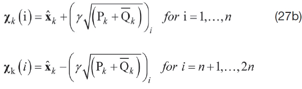
where the matrix ？_k for attitude estimation is related only to the process noise covariance for Eq. (26a). However, Q_k is not the corresponding covariance due to the second term in Eq. (26a). Note

and λ are convenient parameters in taking advantage of whatever knowledge is available of the higher moments of the given distribution. In scalar systems, where n = 1, a value of λ = 2 leads to sixth order errors in the mean and variance that are of sixth order. For higher dimensional systems, choosing λ = 3?n minimizes the meansquared-error up to the fourth order (Banani and Masnadi-Shirazi, 2007; Cheon and Kim, 2007). However, caution is required when λ is negative since the predicted covariance may become a positive semi-definite covariance matrix. Also, when n+λ tends to zero, the mean tends to be that calculated by the truncated second-order filter. The matrix square root

can be calculated by a lower triangular Cholesky factorization (Julier et al., 1995). From Eq. (27), the matrix χk of 2n+1 sigma vectors χi, k is formed as

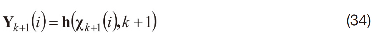
The transformed set of sigma points is evaluated for each of the points by

where χ_k+1(i) is the i^th column of χ_k.The predicted mean x?^?_k+1 and the predicted covariance P^?_k+1 are computed using a weighted sample mean and the covariance of the posterior sigma point vectors as

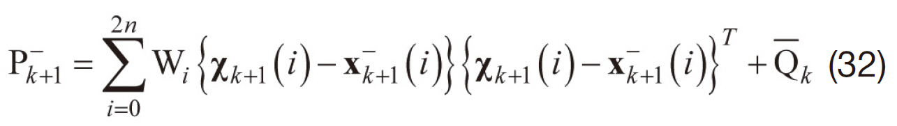
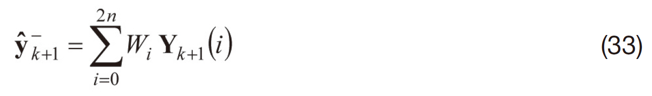
The mean observation is given by

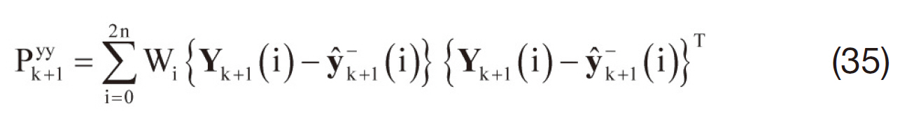
The predicted output covariance P^yy_k+1 is given by

The innovation covariance P^yy_k+r is then computed by

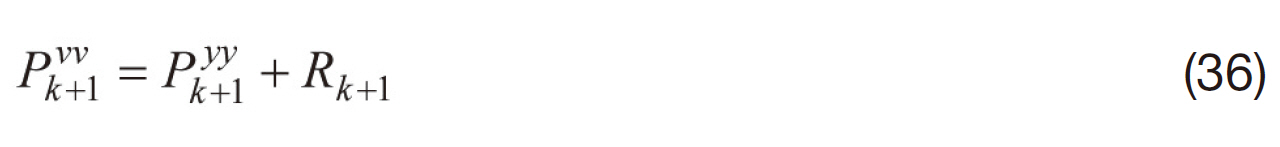
The filter gain K_k+1 is computed by

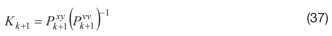
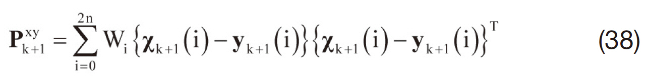
and the cross correlation matrix is given by

The estimated state vector x? ⁺_k+1 and updated covariance P+k+1 are given by

This section shows the derivation of the UKF for relative attitude estimation. In general, the UKF cannot be implemented directly with the equations in Section III because of the violation of the unit quaternion constraint. It is difficult to compute the means of a set of sigma points because the rotation represented by the quaternion does not belong to a vector space, but lies on a nonlinear manifold. Furthermore, the quaternion is constrained to the three-dimensional unit sphere of a four-dimensional Euclidian space. The quaternion predicted mean using Eq. (31) is not guaranteed to maintain a unit quaternion because the quaternion is not mathematically closed for addition and scalar multiplication. This limitation makes the straightforward implementation of the UKF with quaternions undesirable. On the other hand, an EKF can be designed using this approach, in which the quaternion normalization is performed by “brute force.”To use the UKF, an unconstrained three component vector is used to represent the attitude error quaternion. First, the state vector is defined as

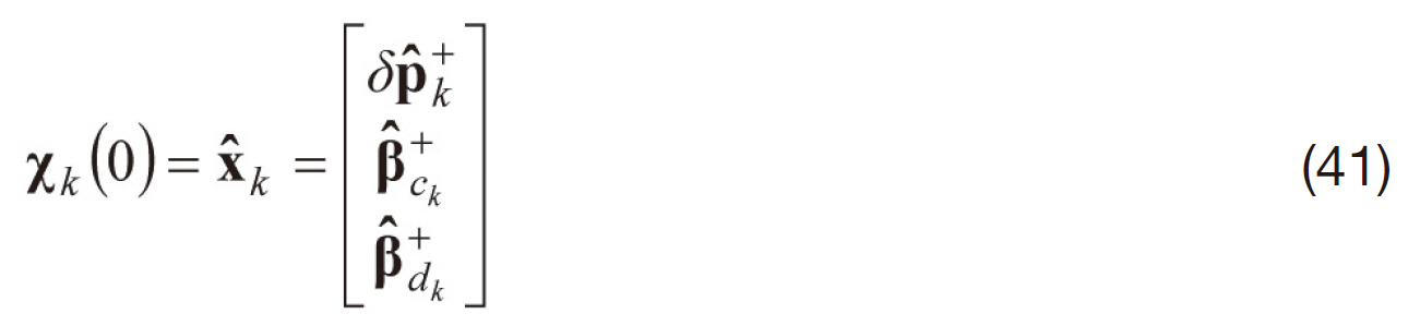
where δp?⁺_k is the updated vector of generalized Rodrigues parameters, and β? ⁺_ck and β? ⁺_dk are the updated gyro bias of the chief and the deputy spacecraft, respectively. Using δp?⁺_k from Eq. (14), the nominal quaternion is propagated and updated. The overall covariance is a 9×9 matrix, and this threedimensional representation is unconstrained. The use of Eq.(31) causes no difficulty, providing an attractive method of attitude representation. First, the vector χ_k(i) in Eq. (27) is partitioned into

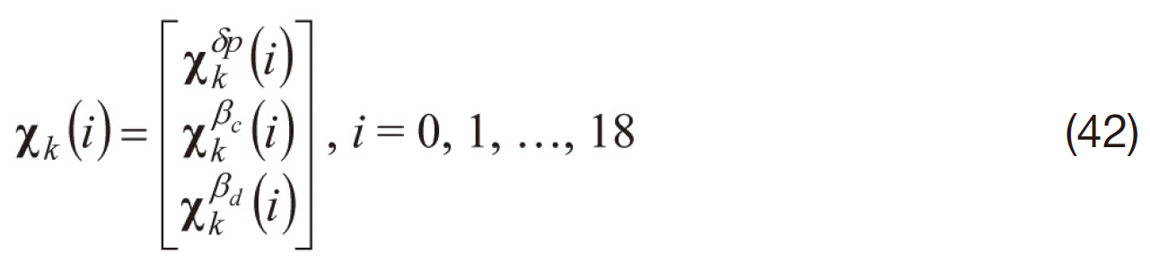
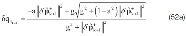
where χ_k^δp is the attitude-error, χ_k^βc(i) is the chief gyro bias and χ_k^βd(i) is the deputy gyro bias. Since the unit quaternion is not closed for addition and subtraction, the transformed sigma points of the quaternion are not simply constructed,while the sigma points for the gyro bias are calculated by Eq.(27). Rather, the transformed sigma points of the quaternion are also quaternions satisfying the normalization constraints and should be scattered around the current quaternion estimate on the unit sphere. Therefore, the transformed quaternion sigma points are generated by multiplying the error quaternion by the current estimate. To generate quaternion samples evenly on the unit sphere around the current quaternion estimate, both the error quaternion and the inverse of the quaternion δq⁺_i,k and (δq⁺_i,k)^?1 are used. The sigma point quaternions are then computed using

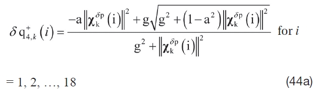
where δq⁺_k (i)=[δρ^+T _kδq⁺_4,k (i)]^T is represented by Eq. (15) as

Eq. (40a) clearly requires that χ_k^δp(0) be zero since the attitude error is reset to zero after the update, and this resetting moves information from one part of the estimate to another part. For the definition of sigma points, the gyro bias part of the chief and the deputy from γ Pk+ Q?k

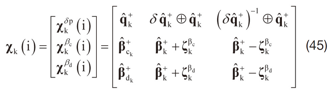
in Eq.(29) are denoted as ζ_k^βc and ζ_k^βd, respectively. The sigma points corresponding to the quaternion actually depend on the quaternion itself, regardless of the chief and the deputy bias.All sigma points are constructed as

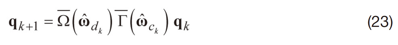
Now these transformed quaternions are propagated forward to k+1 by Eq. (46) as

where the estimated angular velocities of the chief and the deputy are given by Eq. (47) as

Note that χ_k^βc(0) is the zeroth-bias sigma point given by the current estimate χ_k^βc(0)= β?⁺c_k, χ_k^βd(0)= β? ⁺_dk. The propagated quaternion is computed using

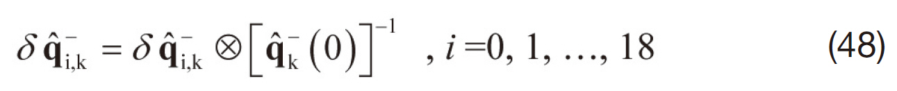
Note that q^??_k(0) is the identity quaternion. Finally, the propagated sigma points can be computed using the representation of Eq. (14) as

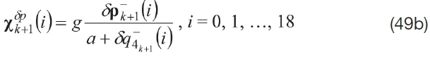
with [δρ^?T _k+1(i) δq^?_4k+1(i)]^T= δq^?T _k+1(i). Furthermore, from Eq.(22b)

The predicted mean and covariance can now be computed using Eqs. (31) and (32), respectively. The output covariance,innovation covariance, and cross-correlation matrices are computed using Eqs. (35), (36), and (38), respectively. Next,the state vector and covariance are updated using Eqs. (39)and (40) with x? ?_k+1=[δp?^+T_k β? ^+T_ck β? ^+T_dk ]^T. The quaternion is then updated using

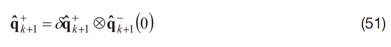
Note that δq⁺_k+1=[δρ^+T _k+1 δq⁺_4k+1]^T is represented by Eq. (15) as

Finally, δp?⁺_k+1 is reset to zero for the next propagation.

This section shows the derivation of the necessary equations for both relative attitude estimation and relative navigation, accounting for relative position and velocity. The state vector in the attitude-only formulations shown in the previous section is now appended to include the relative position and velocity of the deputy, the radius and radial rate of the chief spacecraft and the true anomaly and its rate. This appended vector is given by Kim et al. (2007)

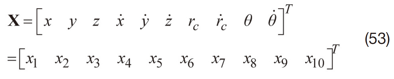
The nonlinear state-space model follows Eqs. (1) and (2)

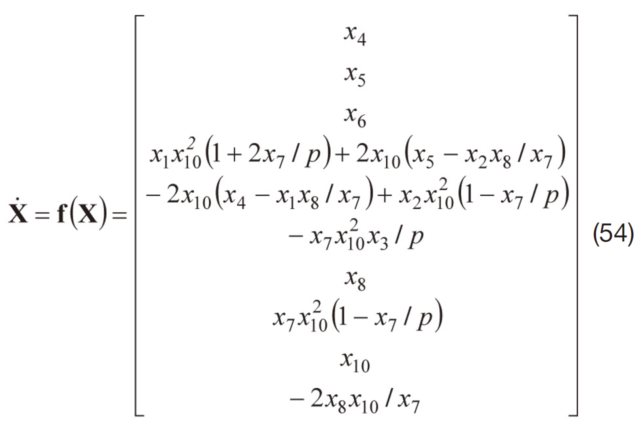
In this formulation, the chief radius and true anomaly are estimated, along with their respective derivatives. If this information is assumed to be known initially, then these states can be removed and their observed values can be added as process noise in the state model. The necessary equations for relative attitude estimation between two spacecraft are derived in Kim et al. (2007). Among the three ways to represent the state presented in Kim et al.(2007) based on the EKF, this work selected the estimation of relative attitude and individual gyro biases for the chief and the deputy spacecraft. From the derived error-state dynamics, the discrete-time covariance matrix is computed and is applied equally to the UKF. The linearization process makes the following assumptions, which are valid to within first-order (Lefferts et al., 1982):

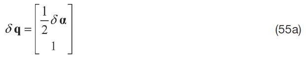
where δα is a small angle-error correction. Then, the errorstate dynamics for the relative attitude estimation is given by Kim et al. (2007)

with

where

and the spectral density matrix of the process noise w is given by

For the estimation of relative attitude and the states in Eq.(53) together, the error-state vector for the chief and deputy gyro bias case is now a combination of Eqs. (53) and (57a)as

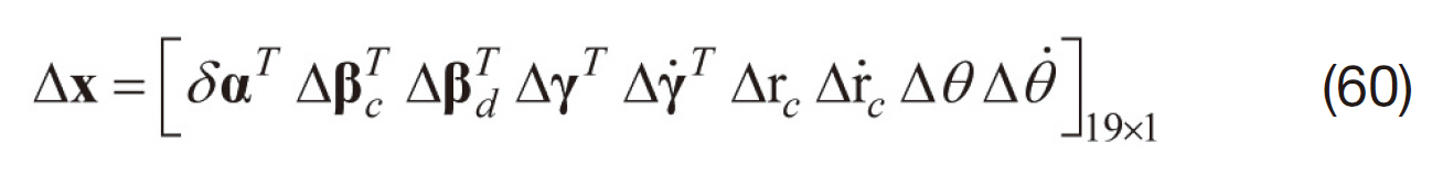
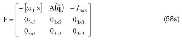
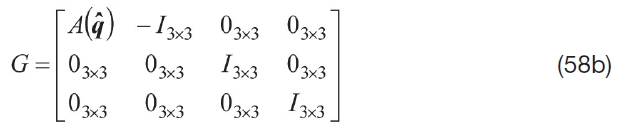
with the obvious definitions of Δγ, Δγ?, Δr, Δr?_c, Δθ and Δθ?.The matrices F and G used in the EKF covariance propagation are also used for the UKF sigma point generation in Eq. (27)and for the predicted output covariance Eq. (35). These augmented matrices are given by

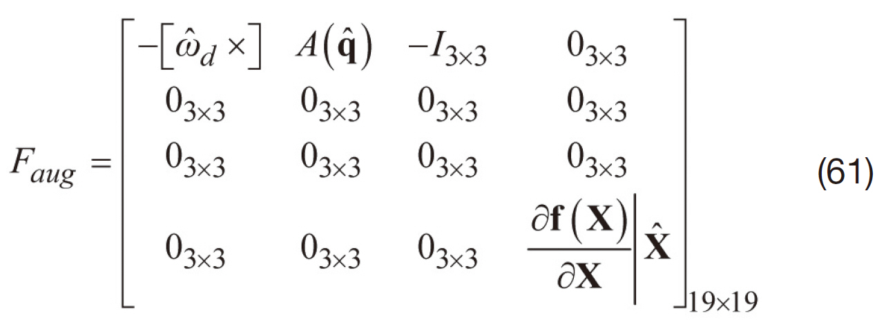
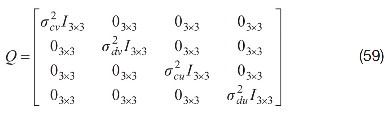
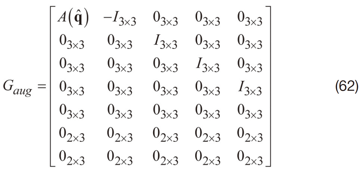
where X？ denotes the estimate of X. The partial derivative ？f(X)/ ？X is straightforward, but for brevity, is not shown here. The augmented matrix Gaug is given by

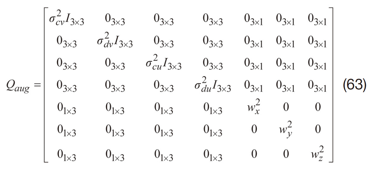
Defining the new process noise vector as w=[η^T _cv η^T _dv η^T _cuη^T _dv w_x w_y wz]^T _15×1, the new augmented matrix Q_aug is given by

Solutions for the state transition matrix F in Eq. (56) and the discrete-time process noise covariance are intractable due to the dependence of both on the attitude matrix (Kim et al., 2007). For the convergence of the state, w_x, w_y, w_z in Eq.(63) should be properly tuned experimentally, considering the scale of the relative disturbances that exist in HPOP modeling. A numerical solution is given by van Loan for fixed parameter systems, which includes a constant sampling interval, the time invariant state, and covariance matrices(Brown and Hwang, 1997; Van Loan, 1978). First, a 38×38 matrix, A?, is formed as

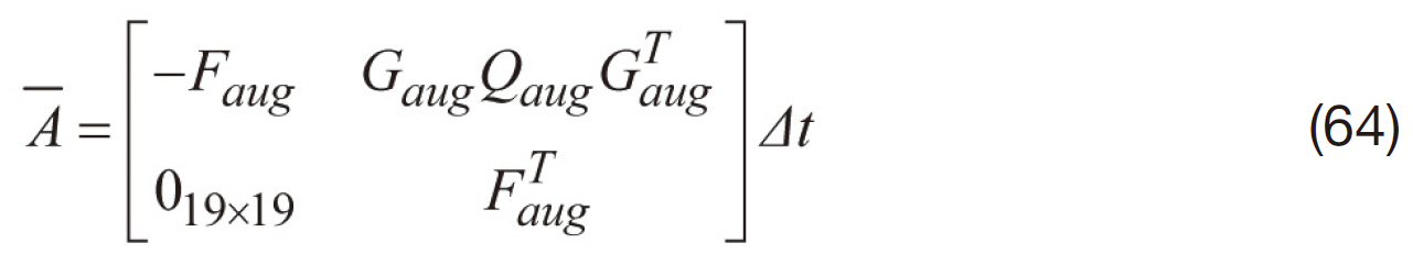
Then, the matrix exponential of Eq. (64) is computed as

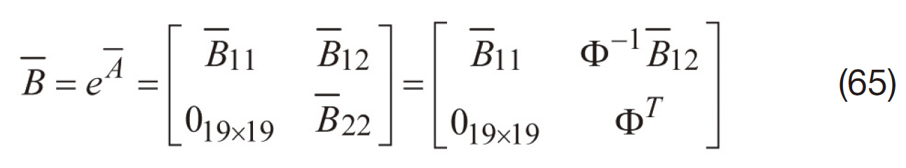
where Φ is the state transition matrix of F in Eq. (56) and Q?_aug is the augmented discrete-time covariance matrix.The state transition matrix and discrete-time process noise covariance are then given by

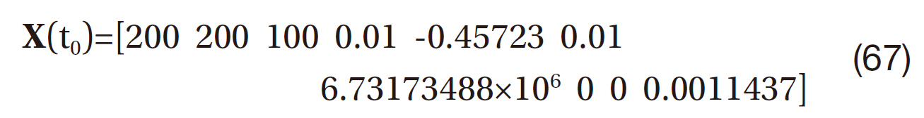
In this section, the performances between UKF and EKF approaches are compared several times through simulated examples using STK for realistic relative navigation between the International Space Station (ISS), which is the chief, and the Space Shuttle, which is the deputy. For this simulation, a bounded relative motion constraint is applied using Eq. (3). The ground tracks and orbits of the two spacecrafts appear almost identical. The scenario begins at the perigee of the chief and proceeds over ten hours of bounded relative motion. The initial condition for the vector X in appropriate units of meters, meters per second, radians and radians per second is given by

The simulation time for the relative motion between the two spacecrafts is 600 minutes, and step size is 10 seconds. The orbit period of the chief is nearly 92 minutes. For the entire simulation, the true relative attitude is simulated by propagating Eq. (23) using an initial quaternion given by

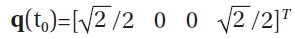
and angular velocities given byω_c=[0 0.0011 ?0.0011] rad/sec and ω_d=[?0.002 0 0.0011] rad/sec. The gyro noise parameters are given by

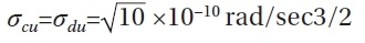
and

(Kim et al., 2007). The initial biases for each axis of both the chief and the deputy gyros are given as 1 deg/hr. Six beacons are assumed to exist on the chief, and their configuration is shown in Fig.2.These beacons are assumed to be visible to the PSD on the deputy throughout the entire simulation run. Simulated VISNAV measurements are generated using Eq. (16) with a standard observation deviation of 0.0005 degrees. Each covariance sub-matrix for attitude, gyro biases, position and velocity is assumed to be isotropic, a diagonal matrix with equal elements.

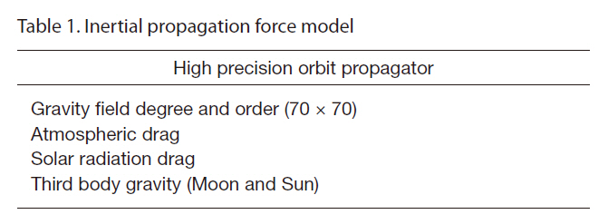
To validate the estimated relative position and velocity, a simulation truth model is generated with Eq. (1) by adding acceleration disturbances to the right side, which are modeled as zero-mean Gaussian white-noise process (Kim et al., 2007). However, this model may not be sufficiently realistic. To address this issue, a high-fidelity propagator may be used instead to generate “true” spacecraft ephemerides. For a more realistic validation, both spacecrafts are modeled with HPOP of STK (Analytical Graphics Inc.) using the force model in Table 1. The simulated truth model is computed using Eqs. (5-9).

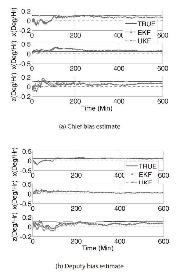
The first simulations with both the UKF and the EKF are performed under ideal conditions, i.e. with no initial attitude errors, initial bias estimates set to zero, and no initial position and velocity errors. The initial attitude covariance is set to P_att=I_3×3(deg)², and the initial chief and deputy gyro bias covariances are each set to ??. P_bias=4I_3×3(deg/hr)², the initial position covariance is set to P_pos=5I_3×3m² and the initial velocity covariance is set to P_vel=0.02I_3×3(m/s)². The initial variance for the chief position is set to 1,000 m² and the velocity variance is set to 0.01 (m/s)². The initial variance for the true anomaly is set to 1×10^?4 (rad)², and the rate variance is set to 1×10^?4(rad/sec)². The gyro and LOS are both sampled at 10 seconds intervals for 600 minutes. Also, α = 1 with g = 4, which gives four times the vector of MRPs for the error representation, and λ = 1 is chosen for these simulations. Figure 3 shows the

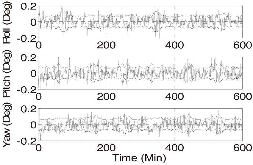
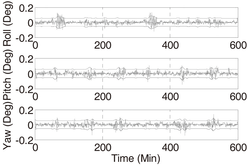
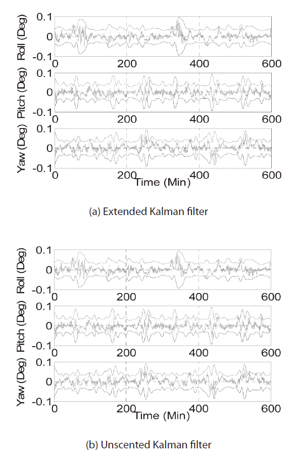
accurate estimation of the chief and deputy biases. Figure 4 shows the attitude errors and respective 3σ bounds derived from the UKF and the EKF.

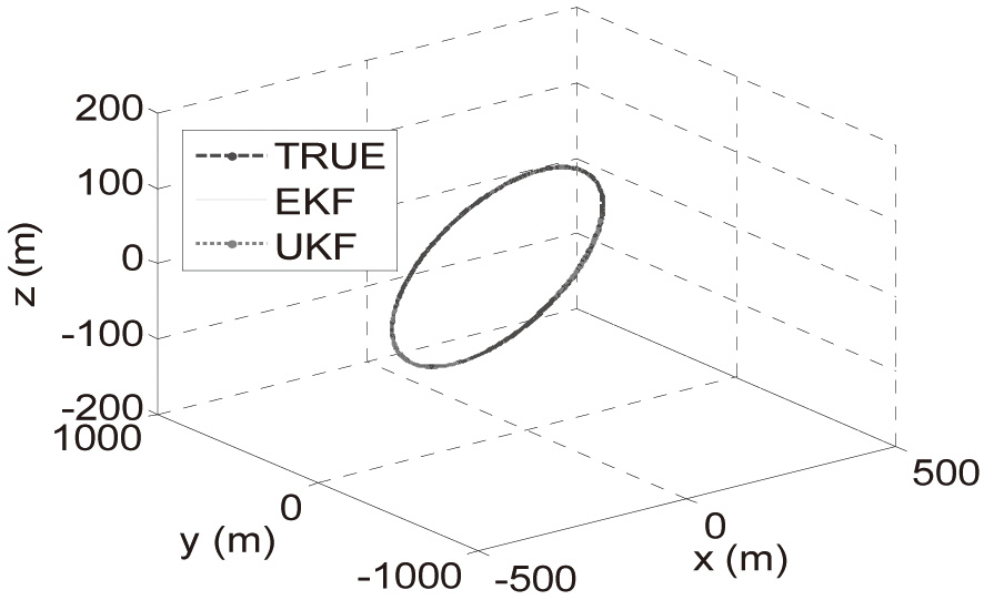
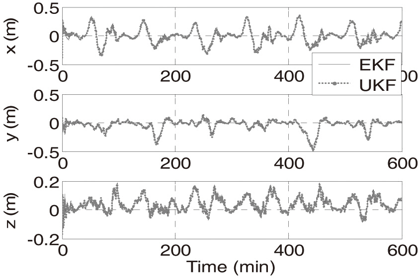
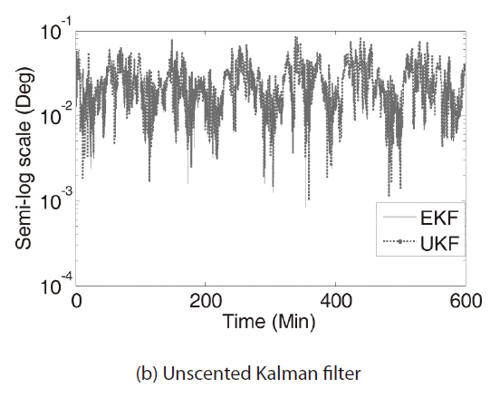
Figure 5 shows that the norm of the attitude errors is less than 10^?1 deg. Figure 6, the estimated relative orbit, shows that the error is bounded by less than ±0.5 m in three-dimensional space.Figures 7 and 8show the relative position and velocity errors. There is no significant difference between the UKF

and the EKF under this ideal condition. These results indicate that the UKF does not give any advantages in this case.

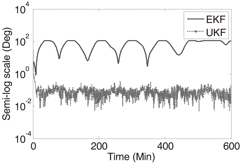
In the second simulation, errors of ?10° in yaw, ?15° in pitch and ?25° in roll are added to the initial condition attitude estimate using Eq. (54), with the bias estimate set to zero. The initial attitude covariance is set to (20 deg)2, and the initial bias covariance is unchanged. Whereas the EKF never converges, the UKF converges to a value below 0.2° in attitude errors and respective 3σ bounds before one period of the chief as shown in Figs. 9 and 10. The attitude estimated by the EKF is not appropriate in this case.

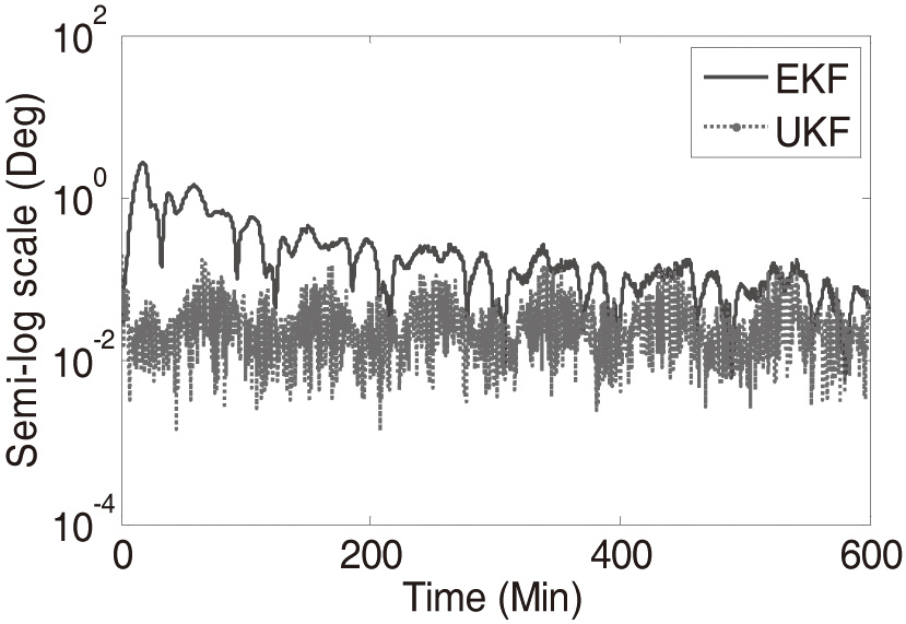
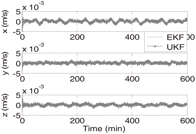
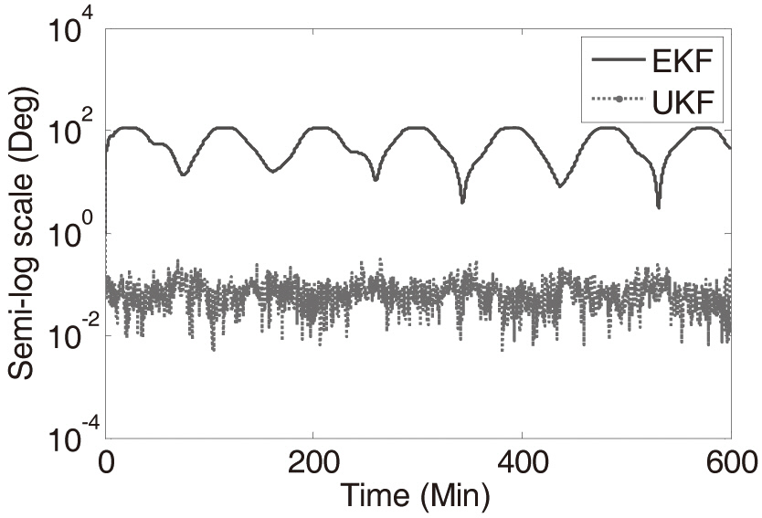
In the third simulation, with initial biases set to zero, the initial attitude error is set to zero. Instead, errors of (10 m, ?10 m and 10 m) are made in the initial relative position and errors of (0.5 m/s, 0.5 m/s and 0.5 m/s) are made to the relative initial velocity. The EKF takes long time to converge. In addition, it never converges to a value below 0.1° in attitude errors and respective 3σ bounds stably as shown in Fig. 11, whereas the UKF converges to a value near 0.1° from the beginning in Fig. 1

The fourth simulation portrays the most realistic situation. All initial attitude, bias, position, and velocity errors are considered together as in the second and the third simulations. The estimation performance of the EKF deteriorates throughout the simulation, whereas the UKF converges to below 0.2 degrees attitude errors and respective 3σ bounds as shown in Figs. 13 and 14. In all these simulations, the UKF demonstrates its robustness under the initial error conditions.

This work extended a previously suggested approach for absolute attitude estimation to relative attitude estimation and navigation of spacecrafts based on the use of the UKF,and evaluated the performance of this extended approach for bounded relative motion to verify its robustness under initial error-conditions. This work also employed the quaternion expression, which was represented by a threedimensional vector of generalized Rodrigues parameters,to maintain a unit quaternion constraint. For estimations of relative attitude, relative position and velocity, the error-state vector was combined. The simulation results using the UKF were compared with those for the EKF. The states estimated by the UKF converged more quickly and precisely with the initial error conditions. The estimated relative position and velocity were validated by comparing them with the state computed from the two orbits generated by HPOP in STK.Thus, the implemented UKF demonstrated its robustness and showed improved estimation results under realistic initial error-conditions. This research shows that the VISNAV system using the UKF can provide precise information on relative attitude, and relative position and velocity under initial error-conditions.