This work addresses problems regarding trajectory planning for unmanned aerial vehicle sensors. Such sensors are used for taking measurements of large nonlinear systems. The sensor investigations presented here entails methods for improving estimations and predictions of large nonlinear systems. Thoroughly understanding the global system state typically requires probabilistic state estimation. Thus, in order to meet this requirement, the goal is to find trajectories such that the measurements along each trajectory minimize the expected error of the predicted state of the system. The considerable nonlinearity of the dynamics governing these systems necessitates the use of computationally costly Monte-Carlo estimation techniques, which are needed to update the state distribution over time. This computational burden renders planning to be infeasible since the search process must calculate the covariance of the posterior state estimate for each candidate path. To resolve this challenge,this work proposes to replace the computationally intensive numerical prediction process with an approximate covariance dynamics model learned using a nonlinear time-series regression. The use of autoregressive time-series featuring a regularized least squares algorithm facilitates the learning of accurate and efficient parametric models. The learned covariance dynamics are demonstrated to outperform other approximation strategies, such as linearization and partial ensemble propagation, when used for trajectory optimization, in terms of accuracy and speed, with examples of simplified weather forecasting.
Many natural phenomena experience rapid change. As a result, regular measurements must be taken in order to determine the current state of a natural system. Natural systems include weather, vegetation, animal herds, and coral reef health. Without frequent measurements, the difference between the estimated state of these dynamic systems and the true state can grow arbitrarily large. Sensor networks have been successfully applied and utilized in many realworld domains in order to automate the measurement process. However, but these domains possess characteristics that may limit how the sensors are deployed. Complete sensor coverage of any real-world domain is impractical because of excessive cost, time and effort. For example, it is considerably easier to deploy permanent weather sensors on land than over open ocean areas. Given finite resources,the amount of sensor information, and therefore the quality of the state estimate, is typically unevenly distributed across the system.
The fast moving dynamics of natural domains present two challenges. Firstly, the state dynamics are strongly coupled, meaning that part of the system can often have farreaching influence on the rest of the system. Secondly, the state dynamics are also chaotic; in other words, very small changes in the current state can lead to very large changes in the future. As a result, if some parts of the system are not sufficiently known and accurately described, the accuracy of the estimated state of the whole system is significantly reduced, as is our ability to produce predictions about the future state.
Additional measurements may improve the accuracy of state predictions. However, given finite resources, only a subset of the state can be measured with additional sensors. For mobile sensors, care must be given to choosing the locations in the system that will maximally reduce the expected error of future predictions. In particular, dynamic system prediction frequently uses a probabilistic form of filtering in which a probability distribution over the state is maintained. If the state is normally distributed with a mean and covariance, the sequence of measurements that minimizes some norm on the covariance is usually preferred.
The path selection problem (or “informative path planning” problem) may be straightforwardly solved if the posterior covariance can be computed efficiently subsequent to taking a sequence of the measurements (Berliner et al.,1999; Choi and How, 2010b). When the system dynamics are linear (and any perturbations to the system or to the measurements are Gaussian), the posterior covariance given a sequence of measurements can be easily and accurately computed using the Kalman filter (EKF). However, when the dynamics are nonlinear, the calculation of the posterior must be approximate. In particular, when the dynamics are chaotic, complex, and of large-scale, Monte-Carlo methods are often used to estimate these nonlinear systems (Furrer and Bengtsson, 2007). The ensemble Kalman filter (EnKF)is one such Monte-Carlo filtering algorithm that has seen intensive use in numerical weather prediction (NWP) and other environmental sensing applications (Ott et al., 2004).
Evaluating a set of candidate measurement plans requires a set of Monte-Carlo simulations as a means for predicting the posterior covariance for each plan (Choi and How,2010b). This process can be computationally demanding for large-scale nonlinear systems because producing an accurate prediction typically requires many samples for predicting the mean and covariance of the system state (Choi et al., 2008). Furthermore, additional measurements, which remain unknown during the planning time, will affect the evolution of the covariance; we need the ability to revise the plan quickly upon receiving new measurements. Therefore,an efficient way of predicting future covariances given a set of measurements is essential to tractable planning of informative paths in large-scale nonlinear systems.
In this paper, we present the trajectory planning of a mobile sensor as a means for improving numerical weather predictions. Our primary contribution is to show that the planning process can be made substantially more efficient by replacing the Monte-Carlo simulation with an explicit model of covariance dynamics learned using a time-series regression. The regressed model is orders of magnitude faster to evaluate within the trajectory optimization. We also show that its accuracy of covariance prediction is better than other possible approximations such as linearization or partial use of the Monte-Carlo samples.
2. System Models and Forecasting
This work considers a large-scale dynamical system over a grid in which each cell represents a small region of the overall system and is associated with state variables representing physical quantities (e.g., temperature, pressure,concentration, wind speed) in the corresponding region.Without loss of generality, it is assumed that only one state variable is associated with a cell. The dynamics of the state variables are described by differential equations (Lorenz and Emanuel, 1998).

where
Knowing the current state of a system st, we can use it as the initial condition for the dynamics in Eq. (1), to compute a forecast of the system state in the future. However, we rarely know the true state of the system, but must take multiple(noisy) measurements of the system state, and use a filtering process to estimate

where h is the observation function, mapping state variables and sensing noise w

where
In order to mitigate the effect of measurement noise, a probabilistic estimate


where the prediction step gives the posterior distribution due to the dynamics, following the system dynamics f=Δ
If
When
The EnKF (Evensen and Van Leeuwen, 1996) (and it variants [Ott et al., 2004; Whitaker and Hamill, 2002]) is a Monte-Carlo (ensemble) version of the extended EKF.Monte-Carlo methods are often used to estimate nonlinear systems, especially when the system dynamics are chaotic,complex, and large-scale (Furrer and Bengtsson, 2007).The EnKF is one such Monte-Carlo filtering algorithm that has seen intensive use in numerical weather prediction(NWP) and other environmental sensing applications (Ott et al., 2004), since it typically represents the nonlinear features of the complex large-scale system, and mitigate the computational burden of linearizing the nonlinerar dynamics and keeping track of a large covariance matrix (Evensen and Van Leeuwen, 1996; Whitaker and Hamill, 2002), compared th the EKF.
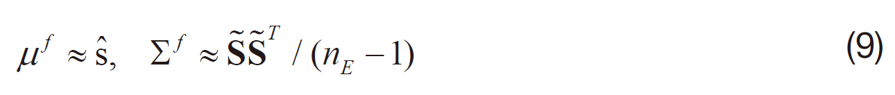
In the EnKF, a set of possible state variable values is maintained in an ensemble matrix S∈ R

where
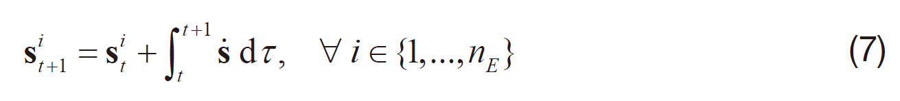
Note that the dynamics integration of an ensemble member involves the integration of

and perturbation ensemble matrix S?, defined as
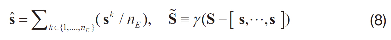
where γ>1 is an inflation factor used to avoid underestimation of the covariance (Whitaker and Hamill, 2002), so that
The measurement update step is similar to that of the EKF,where

A complete derivation of the EnKF is outside the scope of this paper; a full explanation of this nonlinear estimation method can be found in Whitaker and Hamill (2002).
A significant problem existing in current operational systems for environmental sensing is that the measurements are unevenly distributed. Even with a perfect system dynamics model, the forecast of the system may degrade greatly for forecasts made far into the future, as the poor state estimate propagates to other regions over multiple steps of forecasting(Morss et al., 2001). While additional measurements of the initial state estimate will clearly improve the forecast, the number of resources available to take measurements, such as unmanned aerial vehicle (UAV)-borne sensors, is finite.Furthermore, measurements at different locations and times possess different amounts of information due to the spatiotemporal correlations of the state variables. To make the most effective use of finite resources, we must consider the value of the possible measurements in terms of prediction performance (Berliner et al., 1999; Choi and How, 2010a, b;Morss et al., 2001), and choose to measure the state variables that maximize the prediction accuracy.
Adaptive observation targeting has proven to be an important variant for informative path planning. Researchers have maintained great interest in adaptive observation targeting within the context of numerical weather prediction in which the figure of merit is forecast performance at a verification region (Choi and How, 2010b). For example,a goal may be established to take measurements over the Pacific to maximize the forecast accuracy for California, the verification region. The verification region is usually a small subset of the overall system; we denote the cells in this region by
There are also three important times in the weather targeting problem:
Planning time Tp∈Z : the planning starts at Tp.
Forecast time Tf ∈Z : the time at which the last measurement will be taken, and a forecast will be generated. The entire planning, execution and forecasting process must be completed by Tf.
Verification time Tv∈Z : the time at which the forecast will be tested. For instance, a 4-day forecast made at 9th September 2008 (Tf) will be verified at 13th September 2008 (Tv).
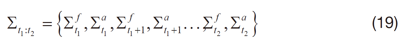
We can write the planning problem formally as

subject to Σ f t+1=F(μat, Σat), ∀t[Tp-1, Tv-1]∩Z
Σat =M(μat, Σf t , pt), ∀t[Tp, Tv]∩Z
Σat=given
where Σ(
Note that the covariance dynamics function
The informative path planning problem in a dynamic system is inherently an NP-hard problem (Choi and How,2010b; Krause et al., 2008), as every possible plan sequence must be evaluated while the number of possible sequences exponentially grow with the length of the planning horizon.Given the large size of the domains under consideration,a multi-scale planning approach may be desired. While finding the global path is computationally infeasible, finding the best local path within a small region may be feasible. Furthermore, there are some planning schemes available,which utilize locally optimal paths that make better choices at higher levels (Choi and How, 2010a). The local path planning task entails choosing the most informative path to move in between two waypoints, maximally reducing the uncertainty in the region between the waypoints. This decision making can also be addressed with the formulation in Eq. (11) by setting
4. Covariance Dynamics Learning
We wish to approximate the

where

where
Since we do not know the exact form of

Specifically, regression is used in order to learn a model with continuous-valued output. Regression learns a target function g given a finite number of training samples;inputs

is expected to have the property

The learning approach aims to achieve accuracy by relying on nonlinear features of the input to represent the complex nonlinear function

and the prediction time of using the learned model
will remain nearly the same, being independent of the accuracy of the training samples (Evgeniou et al., 2000).
In principle, we can learn a predictor of any function of the future covariance; for example, a direct mapping from the current covariance to the trace of the verification subblock of the covariance after

However, we argue that learning the one-step approximator
is the best approach. One has to consider the fact that as the target function becomes more complicated, more training samples and sophisticated features may be required.While generating more training samples only requires more Monte-Carlo simulations, finding sophisticated features requires finding a proper transformation of the original features through many trial and error investigations (Guyon and Elisseeff, 2003). In addition, learning common functions which can be applied for different paths may be preferred.Having learned the one-step approximator
, we can use the approximator to evaluate any path combined with a given measurement update function M(·, ·). In order to predict the covariance multiple timesteps into the future, we can use recursive prediction, in which the output of at time t+1 is used as input at time
will be relatively easier than that of

or other more complicated functions.
4.1 Feature selection: autoregressive time-series mode
The input to the true covariance dynamics
, we select features in order to avoid overfitting and manage computational cost. However, learning with many features creates additional problems since many of the features are noisy or irrelevant; in other words, selecting the most relevant features has led to more efficient learning (Guyon and Elisseeff, 2003). We use the idea of state-space reconstruction(Box et al., 1994; Sauer et al., 1991), a standard methodology for learning nonlinear dynamical systems. The methodology uses time-series observations of a system variable in order to learn the dynamics of the system. The time-series of the observed (specified) variable contains information of the unobserved (unspecified) variables; thus, learning the dynamics only through observed variables is possible.
Following this idea, we used the time-series of the covariance as the only features for learning the covariance dynamics; the covariance dynamics were modeled with autoregressive (AR) time-series features (Box et al., 1994) so that

where Σ
There ar two types of covariances at time
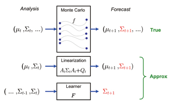
In this way, the effect of the covariance dynamics and the measurement update will be learned altogether. The learning approach is compared to the other methods in Fig. .1
4.1.1 Function decomposition
Because
takes a series of d covariances as input in which each size is

To simplify the learning problem, we decompose
into


The principle of the state-space construction states that this learning problem is solvable as the dynamics of a variable can be learned from the time-series observations of the variable.In addition to the simplicity of learning, decomposition takes into account the locality of the covariance dynamics that the system dynamics
4.1.2. Fast recursive prediction
In many physical systems, the spatially neighboring variables are strongly coupled, and thus their covariances are also expected to be coupled (Furrer and Bengtsson, 2007).Instead of just using the AR features Σ(

we might also use the time-series of the spatially neighboring cells, Σ(
In recursive prediction, all features needed for the next step prediction must also be predicted from the current step.Suppose we want to predict a covariance entry Σ
The entries of
have to be predicted using their own spatial neighbors from Σt. It is easy to see that the number of the entries to be predicted increases with the number of steps in the prediction; the prediction of Σ
and so on. With the use of AR features alone, we only have to know the past values of one covariance entry to predict the next value of the entry.(Editor’s Note: Very well written paragraph)
4.2 Model selection: parametric model learning
In this work, we decided to learn a parametric model of the covariance dynamics, representing
by a linear function of the input x=Σ
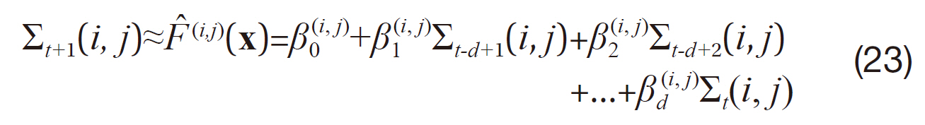
where β(
Eq. (23) models nonlinear or more complicated functions of the original input x by incorporating nonlinear functions of the input features x. For instance, we can transform x=(
The choice of learning a parametric model is to enable faster prediction during the operation. Once the coefficients β(
4.2.1 Regularized least squares regression
Learning of
entails finding the coefficients β(
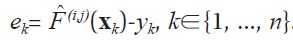
We used regularization to learn
, which did not overfit to the training samples (Evgeniou et al., 2000). Overfitting models may offer zero prediction error by perfectly fitting the training samples; however, such a procedure poorly predicts a new example x*, where x*≠x
Regularization provides extra information from domain knowledge by placing a prior over the regression coefficients β; for example, the L2-norm of the coefficients │β│2 is preferred to be small, as largr │β│2 indicating that the learned function is less smooth and may be the result of overfitting the training samples. The regularized least squares (RLS) algorithm minimizes the sum of the squared-error of the training samples and a regularization penalty,

where λ is regularization parameter which controls the contribution of the L2-norm of regression coefficients β to the total loss function; a larger value of λ encourages smaller │β│2. To minimize Eq. (24), we set the derivative of Eq. (24) with respect to β to 0, and get

We find

for each approximator
using the RLS algorithm, while λ(
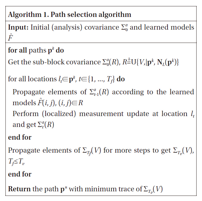
4.3 Path selection with learned covariance dynamics
Once we have learned the models
, we can predict the uncertainty of the system after taking a series of observations, using the learned models and the measurement update function. Specifically, we want the prediction for a region of interest, such as a verification region. Let R represent the cells that correspond to the region, then the number of system variables contained in those cells, i.e., │R│, is typically significantly smaller than the number of state variables,
Full-propagation needs to integrate each ensemble member, as in Eq. (7). Each ensemble represents nS state
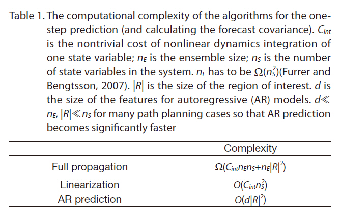
The computational complexity of the algorithms for the onestep prediction (and calculating the forecast covariance). Cint is the nontrivial cost of nonlinear dynamics integration of one state variable; nE is the ensemble size; nS is the number of state variables in the system. nE has to be Ω(nS2)(Furrer and Bengtsson 2007). │R│ is the size of the region of interest. d is the size of the features for autoregressive (AR) models. d≪nE │R│≪nS for many path planning cases so that AR prediction becomes significantly faster
variables, and the integration of one ensemble member takes
However, the learned model calculates each entry of Σ
For the measurement update function, we can use a localized measurement update for further computation reduction, which ignores spurious correlations between two variables that are physically far from each other (Houtekamer
and Mitchell, 2001); for a measurement at location p, only the physical neighbors NL(
In this work, we used the Lorenz-2003 weather model(Lorenz, 2005) for all experiments and for method validation.The Lorenz models are known for their nonlinear and chaotic behavior, and have been used extensively in the validation of adaptive observation strategies for weather prediction (Choi and How, 2010a; Leutbecher, 2003; Lorenz and Emanuel,1998).
The Lorenz-2003 model (Choi and How, 2010b) is an extended model of the well-known Lorenz-95 model (Lorenz and Emanuel, 1998) that addresses multi-scale features of the weather dynamics in addition to the basic aspects of the weather motion such as energy dissipation, advection, and external forcing. We used the two-dimensional Lorenz-2003 model, representing the mid-latitude region (20-70 deg) of the northern hemisphere. There are
We used a two-dimensional index (
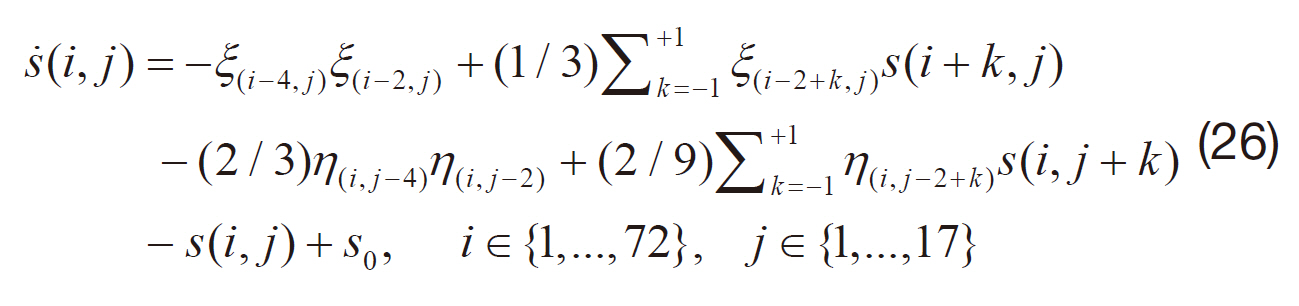
where ξ(
5.2 Covariance dynamics learning results
Table 2 shows the prediction performance of the learned covariance dynamics using different features, while the RLS algorithm was used for all features. The one-step prediction of covariance using the learned models was compared to that of using the true covariance dynamics from Monte-Carlo simulations. The metric used for the prediction performance was the normalized mean squared error (NMSE), which is the MSE normalized by the total variance of the predicted variable. The MSE can be small, even with poor learned models, when the predicted variable exhibited very small variance. The NMSE does not have this problem. The models were trained with a set of training samples and tested on a separate test set in order to measure how well the learned models generalized to the new samples. The values in Table 2 show the prediction errors on the test set.
The AR features containing different degrees, the quadratic and cubic basis expansions, and the spatial neighbors features were compared. Based on the comparison, we clearly observed that the covariance dynamics was better modeled with more complicated models using higherdegree AR features and the basis expansion of the original AR features. The spatial neighbor features also helped prediction performance, but were less useful than the basis expansion of the AR features. It also has the disadvantage of the slow recursive prediction. Note that the number of features increased with the basis expansion; if the original features were AR features with degree d, the full quadratic expansion increases the number of features to
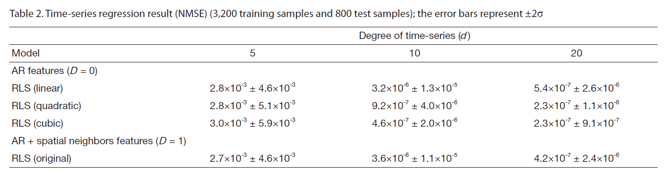
Time-series regression result (NMSE) (3200 training samples and 800 test samples); the error bars represent ±2σ
models with full quadratic expansion can be 20 times slower than the models with original features when d = 20. Thus, we did not use the full basis expansion and added only a few interaction terms to the model.
In accordance with the results, we chose
We compared the accuracy of the learned covariance with other approximation methods and the true covariance dynamics from Monte-Carlo simulations. The partial propagation uses only a random fraction of the original Monte-Carlo samples, which gives a constant factor speedup as the prediction time is linear to the number of the Monte-Carlo samples; if we use 10% of the samples, we get a speed-up of about 10 times that of the original simulation.Note that, however, the computation time of the partial propagation scales with the size of the dynamical system,unlike the learned dynamics case, as in Table 1.
The prediction of the trace of the sub-block covarianceΣ(
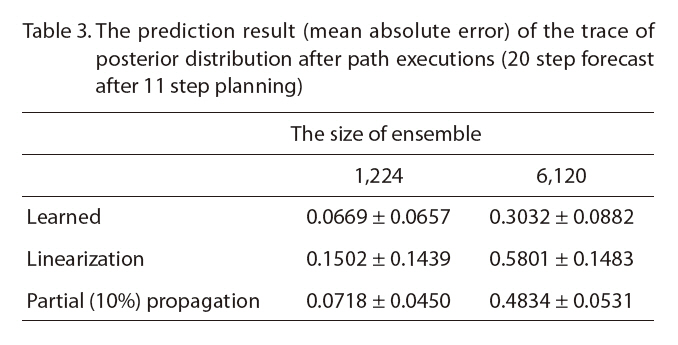
The prediction result (mean absolute error) of the trace of posterior distribution after path executions (20 step forecast after 11 step planning)

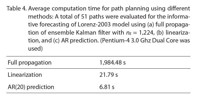
Average computation time for path planning using different methods: A total of 51 paths were evaluated for the informative forecasting of Lorenz-2003 model using (a) full propagation of ensemble Kalman filter with nE = 1224 (b) linearizationand (c) AR prediction. (Pentium-4 3.0 Ghz Dual Core was used)
of mean prediction error, especially with a bigger original ensemble, but had smaller prediction error variance.
The path selection requires the accurate relative ranking of the candidate paths. For that purpose, both the prediction error (bias) and the variance should be small. Roughly,the bias may cause consistent error in the ranking and the variance causes the occasional error in the ranking. We show the path selection result in the next section.
Given the ability to predict the change in covariance of the EnKF efficiently, we can now use the learned function to
identify sensor trajectories that maximize information gain for some region of interest. We assume that a UAV moves from one cell to another of the eight neighboring cells at certain timesteps, taking a measurement at every cell it visits. The system also has a fixed observation network, where about 10 percent of the system is covered by the routine observation network that provides measurements in a regular interval(5 timesteps for this work). We tested two path planning scenarios: adaptive targeting and local path planning. The measure of information gain is the change in the trace of the R sub-block of the covariance Σ(R). R is either a local region or a verification region depending on the planning problem.
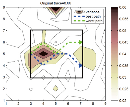
A sample scenario of the local path planning is given in Fig. .3 We considered the case where R is a 5 × 5 local region and the planning horizon is 5. Given the initial state of the EnKF, an agent plans to observe a sequence of 5 locations,one for every timestep, before arriving at the end point. We fixed the start point and used three choices for the end point,thus there were a total of 51 paths in this case. The best and worst paths are illustrated in Fig. .3 In terms of information gain, the best path decreased the trace of the covariance of the region by 15% while the worst path actually increased the trace 1.5%. The average reduction of the uncertainty was 8.3% with standard deviation of 4.6% for 51 paths.
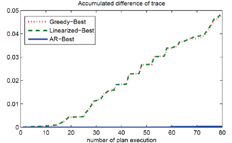
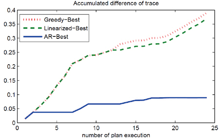
Under the same scenario, we tested the path selection ability of different strategies. The baseline greedy strategy is to choose the path with maximum uncertainty reduction in the current covariance using the measurements; it does not propagate the uncertainty in time and but performs measurement updates on the current covariance. The results of local path selection is shown in Fig. .4 The AR strategy makes almost no mistakes in this case, and the greedy strategy performs similarly to the linearization method. The actual computation time in the experiment is shown in Table .4 The AR prediction was much faster than full propagation and was also faster than linearization. This computational advantage was also theoretically proven with a lower time complexity of the algorithm as in Table .1 The computational advantage will be even greater in larger dynamical systems with bigger Ns than the Lorenz-2003 model.
The other scenario was the targeting problem in the 11 × 11 region near the verification region in Fig. 1,and the reduction of the trace of 20-step forecast (the verification time was 20 steps after the forecast time) was evaluated. There are about 8,000 possible paths, but we randomly selected 100 paths for our experiments; we may not have chosen the true best path,as it may be one of the other 7,900 paths, but the relative performance of the strategies should not be affected by this random selection. The result of the path selection using different strategies is shown in Fig. .5 The prediction result of the learned covariance dynamics enabled the selection of the path close to the true best path of the EnKF.
This paper presented a learning method that improves computational efficiency in the optimal design of sensor trajectories in a large-scale dynamic environment. A timeseries regression method based on autoregressive features and a regularized least-squares algorithm was proposed to learn a predictive covariance dynamics model. It was empirically verified that the proposed learning mechanism successfully approximated the covariance dynamics and significantly reduced the computational cost in calculating the information gain for each candidate measurement path.In addition, numerical results with a simplified weather forecasting example suggested that path planning based on the presented learning method outperformed other approximate planning schemes such as linearization and partial Monte-Carlo propagation.