Geostationary satellites are located at an altitude of approximately 35,786km above the equator, and revolve in the same angular velocity as earth. Geostationary satellites can therefore, communicate with a ground earth station at all times. However, geostationary satellites also experience communication failure time, twice a year, closely one upon the other in spring and autumn quarters. The communication errors occur when ground station-satellite-the Sun are aligned closely, which occurs during spring and fall equinoxes. At such times, thermal noise emitted from the Sun's surface hits the rear side of the satellite and flows directly into the earth station antenna. This is called solar interference. Studies on duration calculation methods and prediction results of a solar interference phenomenon were implemented by many scientists (Vuong & Forsey 1983, Mohamadi & Lyon 1988, Lin & Yang 1989) abroad, and also by Lee et al. (1991) in Korea. To calculate the time of solar interference, information on precise position of the Sun and earth station antenna systems is necessary. Previous researches used the formula of Van Flandern (Van Flandern & Pulkkinen 1979) when calculating the Sun's position, but it has position error of about 1 arcmin. Using the precise ephemeris DE406, which published by NASA/JPL and the earth ellipsoid model, the study calculated the precise positioning of the Sun as causing error within 10 arcsec. For the verification of the calculation, we used TU media ground station located in Seongsu-dong and the MBSAT satellite operated by TU media.
2. Calculation method for coordinates of the Sun
In order to obtain the coordinates of celestial bodies belong to the solar system, the equation of motion of the entire solar system should be solved, and relative equations of motion of solar system bodies used in DE406 is shown in formula (1). (Standish et al. 1992)
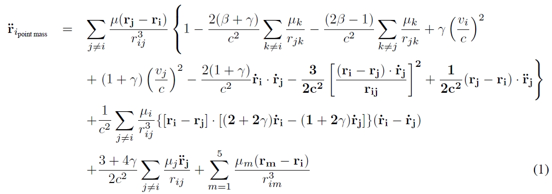
Here, ri, ri and ri represent location, speed and acceleration of the celestial body
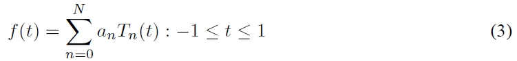
DE406 solves Formula (1) numerically; obtained the computed value by fitting, using Chebyshev polynomial (Newhall 1989), and saved the coefficients in 64 days interval.
The recursion formula of Chebyshev polynomial can be displayed as shown in formula (2).

Here,
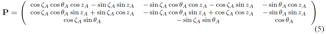


where, ζA,

Since the vector is shown as three-dimensional Cartesian coordinate, semi diameter of the actual Sun as viewed from the earth can be calculated using formula (11) (Meeus 1998).
where,
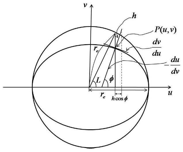
Suppose we are to display the position Re of observers positioned at geographical coordinate (


where,

Formula (16) is obtained when cos
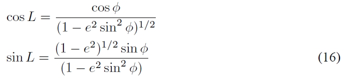
Therefore, using formula (16), the observer position of altitude above sea level h,


where,

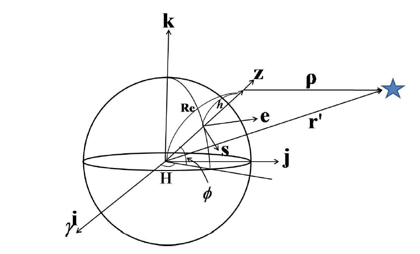
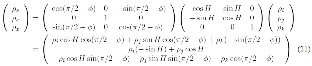
As shown in Figure 2, we can illustrate formula (20) suppose we calculate the position vector ρ from observation place to the Sun, using the vector r', which is the distance between the Sun and center of the earth, and observer postion vector Re.

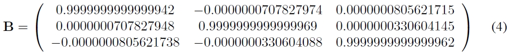
As the vector ρ displayed in three-dimensional geocentric Cartesian coordination, coordinate conversion is required for the 3-axis H and 2-axis (π/2 - φ) direction. This can be illustrated in coordinate transformation matrix as shown in formula (14).
If the vector ρ is conversed to spherical coordinate, we can obtain the azimuth angle and the altitude of the Sun from an observation place. In addition, we calculate an off-axis angle (θ0) between the position of a satellite and the current position of the Sun as formula (22), it is feasible via cosine law of spherical triangle (Lee et al. 1991).

where,
3. Solar Interference Calculation
Antenna noise temperature is proportionate to the ratio of which apparent solar temperature and the Sun is included in the antenna beam. Therefore, to calculate antenna noise temperature, gain pattern of earth station antenna, showing the antenna beam and apparent solar temperature, should be defined.
As the gained pattern changes depending on the characteristic of each earth station antenna, calculation should be obtained through directive measurement. However, obtaining characteristics by measuring each antenna would be practically impossible, thus, the study was conducted based on the WARC-79 gain pattern (CCIR 1982), employed by ITU. The WARC-79 gain pattern has a parameter in accordance with the radio frequency transmitted to antennas and the diameter of antennas.

where,
Hence, the solar noise temperature observed from actual earth station antennas is as shown in formula (25).

Moreover, as the increase of noise temperature in accordance with solar is proportionate depending upon how much solar disc comes into the range of the antenna, thus, it can be integral as formula (26) (Mohamadi & Lyon 1988).

where,
Formula (26) above can integrate simple solar disc, such as on φ direction, hence, it can be converted to an integration method as shown in formula (27) for θ direction (Lin & Yang 1989).

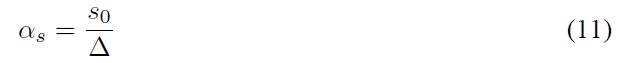
where, αs is 'semidiameter of the Sun', obtained from formula (7), θ0 is 'off-axis angle' obtained from formula (15), and φi is as follows formula

where, αs is 'semidiameter of the Sun', obtained from formula (7), θ0 is 'off-axis angle' obtained from formula (15), and φi is as follows formula
To compare the calculated antenna noise temperature with actual observed value, a barometer enabling quantitative comparison is required, thus, ∠(C/N) is defined as a barometer as follows (Vuong & Forsey 1983, Lin & Yang 1989).

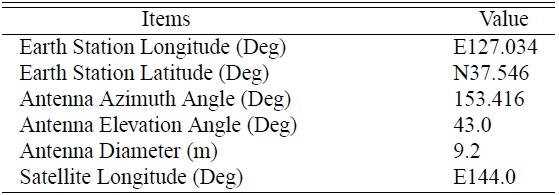
[Table 1.] TU Media Ground Station Information.

TU Media Ground Station Information.
In formula (29),
4. Comparison and error analysis of solar interference time
A calculation program is created for solar interference based on the aforementioned formulas. The Visual C++ .Net 2008 was used for programming, and the Origin program was utilized to simulate graphics. In addition, we calculated the solar interference time of TU media ground station in Seongsu-dong displayed in Table 1, to verify the accuracy of the program, and compared with actual observed value.
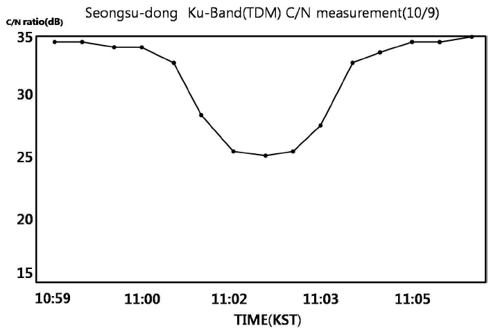
The actual C/N value and time observed from TU media ground station on Seoungsu-dong on October 9, 2007 is illustrated in Figure 3. As of an observation result, the time of solar interference commenced at about 11h01m a.m. on KST, of which reached its maximum at 11h02m30s a.m., and over at about 11h04m a.m.. ∠(
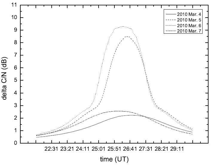
Figure 5 is a graph demonstrates the time of solar interference expected in spring quarter of 2010. According to Figure 5, solar interference starts between 5th and 6th of March, in the case of spring quarter in 2010, and the occurrence time is between 11h24m a.m. - 11h28m a.m.. Solar interference occurs the most in March 6, while maximum interference time is at 11h26m19s a.m., and the maximum ∠(
An error analysis is implemented based on March 6, 2010. The date is forecasted as the day, which most solar interference would occur in the spring quarter of 2010. The maximum solar interference occurred time on this day was at 11h26m19s a.m., and based on the MBSAT satellite information and earth station antenna illustrated in Table 1, we calculated solar interference occurrence time according to each error, and compared the time, which maximum solar interference occurred, and compared with ∠(
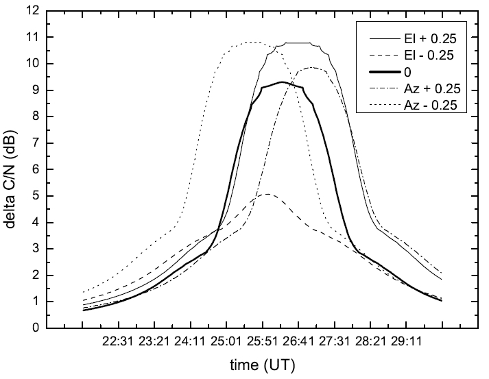
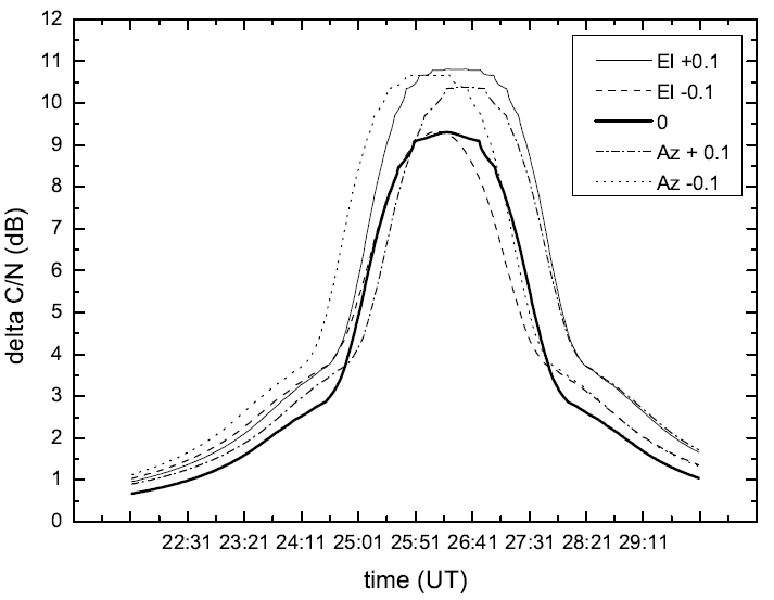
Figure 6 represents when the error of direction of an antenna shows 0.1o. The maximum time of solar interference occurs 9 seconds faster than 11h26m19s a.m. when the altitude of an antenna is lower than the standard altitude 0.1o. When the azimuth angle is as little as 0.1o, the maximum solar interference occurs 35 seconds faster. When altitude is increased by 0.1o, the maximum interference occurs 13 seconds faster, and when, azimuth angle is increased by 0.1o, the interference occurs 16 seconds later. Through this, we are able to confirm that when the altitude of an antenna changes by 0.1o, there is an error range with solar interference time at -35 ∼ +16 seconds. Figure 7 shows the difference when 0.25o error is given to an antenna. The time of maximum solar interference when altitude is as little as 0.25o, it occurs 22 seconds faster than standard time, and when azimuth angle is as big as 0.25o, it occurs 41 seconds late. Thus, suppose we calculate the rest, when the error of bearing of an antenna is 0.25o, we are able to confirm an error range of -27 ∼ +41 seconds.
When we examined Figure 6 and 7, we can see that the intensity of maximum solar interference changes when antenna error occurs, and that changes in the width of ∠(
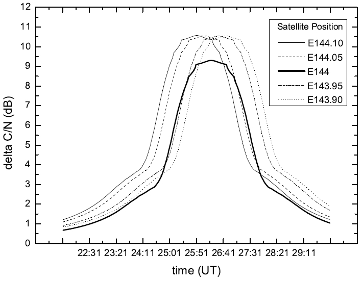
Figure 8, illustrates the change in solar interference time when the position of geostationary satellite changes according to perturbation. Suppose we examine Figure 8, when the position of a satellite moves to east by 0.05o, that is when it is located at the latus rectum 144.05o, the maximum interference time is 11h26m05s a.m., which is faster by 14 seconds compare to when it is positioned at the latus rectum 144.0o, the standard position. When a satellite moves to west by 0.05o and positioned at 143.95o east, the time of maximum solar interference is 11h26m32s a.m., which is 13 seconds delayed than that of standard position. The change of maximum interference period according to the position of a satellite is 0.05o, and has error range of -14 ∼ +13 seconds at the time of change. However, in a case where there is more than 0.1o position change, an error occurs with range of one minute or more. In addition, we can also check the change of intensity of solar interference. However, unlike the error occurrence of antennas, we recognized that there is no significant change of in respective cases when a satellite's position changes.
The purpose of this study is to forecast precise prediction of solar interference time. The study calculated the precise position of the Sun, using DE406 and an earth ellipsoid model, and via a solar interference program, we predicted noise temperature and C/N decline of earth station antenna in accordance with solar interference of stationary satellite and earth station. As a result of applying a communication satellite ground station in Seongsu-dong and MBSAT operated by TU media, we confirmed that they are consistent with actual observation, and verified their accuracy through error analysis.
In-depth of consideration is needed for the intensity of solar interference, not only the affect of the Sun, but also on the specific system of each earth station antenna. Specifically, the size of antennas and a wavelength range of radio wave used in antennas affect the most in the time of solar interference, thus it is necessary to have precise information for a better and precise prediction.
An error according to the position change of a geostationary communication satellite will result a time difference within 30 seconds, if position maintenance is implemented within ±0.05o. Therefore, we expect there will be no significant affect as practical purposes in precise position calculation of satellites. On the other hand, since the direction of antennas can be a significant error factor, precise calculation of the direction of antennas is imperative to the prediction of solar interference time.
In the study, we calculated the time of solar interference between geostationary communication satellite and earth station. In a case of general low orbit satellite, a solar interference time calculation can be conducted using the same method the study employed, if satellite altitude and azimuth angle is obtained from earth station through the orbital elements of satellites.
Moreover, even the precise position of the Moon can be calculated using DE406. It is known that there is noise of about 250K in the Moon, and the interference time according to the Moon can be calculated by taking advantage of this study.