Random fluctuations of fiber birefringences cause polarization- mode dispersion (PMD) effects detrimental to high bit-rate channels. The PMD effects can be described using a PMD vector whose magnitude is equal to the differential group delay between two principal states [1], [2]. When there are many optical channels or the channel bit rate is high, the angular frequency derivative of the PMD vector becomes also important [3]. Often, the conventional PMD vector is called the first-order PMD vector while its angular frequency derivative is called the second-order PMD vector.
In [4], Foschini and Shepp derived a joint characteristic function for two white Gaussian vector processes in a compact functional form using a sine-cosine Fourier expansion representation. The joint characteristic function is a Fourier transform of the joint probability density function (pdf) of two vector processes. Shortly after [4], it was shown that, when the fiber transmission distance is large, the joint characteristic function can be used for the first- and second-order PMD vectors in highly birefringent fibers [5]. This joint characteristic function has been used extensively to describe various distribution characteristics of PMD vectors [6-8]. The birefringence vector model used in [5] assumes a fixed linear birefringence with much smaller linear and circular random birefringences in equal amounts. Interestingly, the joint characteristic function of [5] agrees with the result of [9] that uses the model of [5] without the fixed linear birefringence component. However, installed optical fibers are almost linearly birefringent [10]. Thus it is worthwhile to justify the joint characteristic function of [5] for installed fibers.
Regarding the birefringence components as white Gaussian processes, a Fokker-Planck equation [11] was derived in [12] to investigate the pdf behavior of the first-order PMD vector in linearly birefringent fibers. The Fokker-Planck method was used also in [13] to find a more correct joint characteristic function for the birefringence vector model of [9]. The second-order angular frequency derivative of the fiber birefringence vector was included in [13] but was neglected in [5] and [9]. The birefringence vector distribution of [9] and [13], having linear and circular random birefringences in equal amounts, has a spherical symmetry in Poincare space. This symmetry helps to find the joint characteristic functions of [9] and [13]that are dependent only on the magnitude of two PMD vectors and the angle in between in their Fourier domain. However, the spherical symmetry does not hold for installed optical fibers and, to our knowledge, the joint characteristic function for installed optical fibers is still unknown.
In this paper, we find the joint characteristic function for installed optical fibers. We use the Fokker-Planck method and include the second-order angular frequency derivative of the fiber birefringence vector. Our final result obtained after a complicated procedure has a compact functional form similar to the previous joint characteristic functions [5, 9, 13].
At first, we will present details of the Fokker-Planck method of [12] along with a new shortcut procedure for finding the pdf of the first-order PMD vector. Then we extend the approach to find a Fokker-Planck equation (in Fourier domain) for the first- and second-order PMD vectors. The asymptotic solution of our Fokker-Planck equation yields the joint characteristic function.
II. PDF FOR THE FIRST-ORDER PMD VECTOR
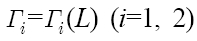
The dynamical PMD equation,
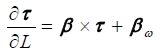
describes the evolution of the first-order PMD vector, τ =(τ 1, τ 2, τ 3) along the fiber [1]. L is the fiber transmission distance. β is the birefringence vector and βΩ=∂β /∂Ω, where Ω is the angular frequency. For linearly birefringent fibers, we set
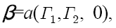
where
is a zero-mean white Gaussian process having a correlation property,

denotes the ensemble average and δij is the Kronecker delta. This modeling neglects the spatial size of the correlation length compared with the large parameter
etc.
We note that the vector equation (1) is composed of three Langevin equations,
where
Then we find the Fokker-Planck equation as follows [11]:
where
From these relations, we have
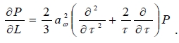
The Fokker- Planck equation for the first-order PMD vector is given by
where
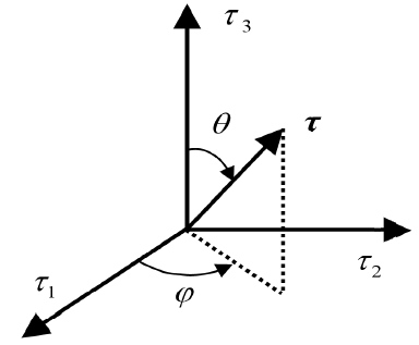
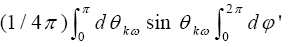
As is shown in Fig. 1, we use a spherical coordinate using the following transform relations [14]:
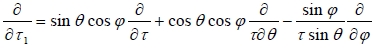
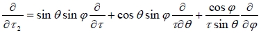
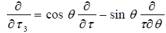
The positive τ 3-axis is the polar axis. θ and φ are polar and azimuth angles, respectively. Since our problem is invariant to the rotation about the τ 3-axis, we may set ∂/∂φ=0. Then the differential operator
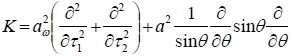
This equation implies that (5) is a diffusion equation along τ 1, τ 2, and θ directions. Therefore, in the asymptotic region, where the transmission distance
We expand
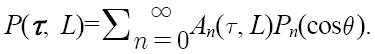
The n-th order Legendre polynomial,
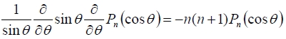
Since
To find
Next, we remove the terms in
Thus, in the asymptotic region,
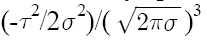
with a variance σ2(
We have used the same initial condition,
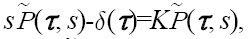
where

is the Laplace transform of
with respect to
III. JOINT CHARACTERISTIC FUNCTION FOR THE FIRST-AND SECOND-ORDER PMD VECTORS
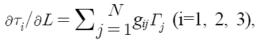
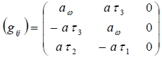
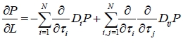
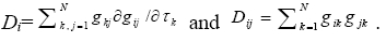
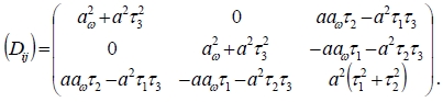
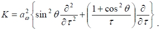
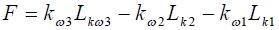
From (1), we find a differential equation for the secondorder PMD vector, τω=?τ/?ω=(τωl, τω2, τω3), as follows:
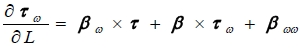
where βωω=?2β /?ω2=aωω(γ1, γ1, 0). We note that (1) and (14) can be regarded as six Langevin equations, ? ? =
where
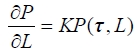
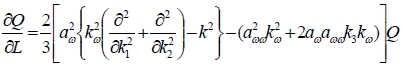
We will solve the Fokker-Planck equation in the Fourier domain by introducing a joint characteristic function,

where
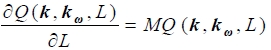
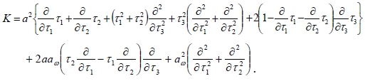
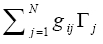
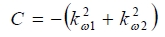
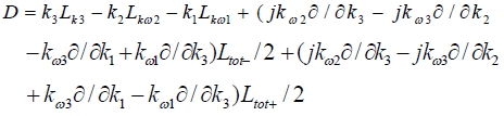
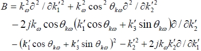
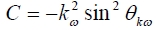
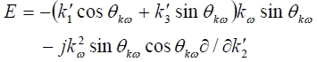
where the differential operator


In (18), we have introduced angular momentum operators defined as
As is shown in the Appendix A, we can find
Since
The

From (24), we find
To find the asymptotic solution satisfying this condition, let's assume that the
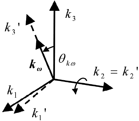
The corresponding rotation matrix is
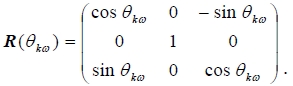
where θωk is the polar angle of
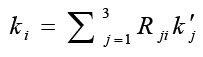
and
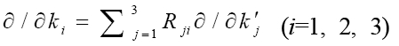
to
In the transformed (
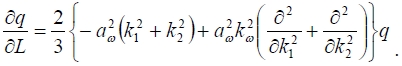
on
Finally, we obtain the following differential equation for the asymptotic solution:
where we have omitted the prime notation. As before, the initial condition remains the same,

where
Equation (31) can be solved using the separation-of-variables method as
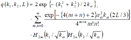
where
we find
Thus, for an arbitrary direction of
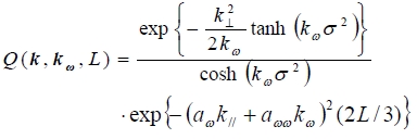
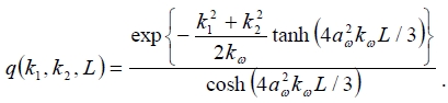
where σ2 =
In the limit of large
With the

condition, the first-order PMD vector distribution has an azimuthal symmetry for all L in [12]. However, the azimuthal symmetry is not evident in our analysis of joint-characteristic function where the number of variables is doubled from 3 to 6. In fact, our final asymptotic solution (35) has spherical symmetry. The coordinate orientation does not affect our result. This kind of spherical symmetry for the asymptotic joint-characteristic function is also found in [5], [9], and [13].
It is also interesting that (35) is quite similar to the result of [13]. The only difference is the change of

is also a zero-mean white Gaussian process having a correlation property,

Note that the number of random birefringence components is larger than our case. Thus, for given
We have found a joint characteristic function for the first- and second-order PMD vectors in installed fibers. As the fiber transmission distance increases indefinitely, our joint characteristic function resembles that of [5] obtained for highly birefringent fibers. This agreement may not hold for practical transmission distances owing to the secondorder angular frequency derivative of the fiber birefringence vector included in our analysis. As an example, we have shown that the second-order PMD vector components can be Gaussian-like distributed instead of a soliton shape. If the fiber length is scaled by a factor of 2/3, our result obtained for linearly birefringent fibers has the same functional form with the previous joint characteristic function of [13] obtained for fibers having a spherically symmetric birefringence vector distribution in Poincare space.