A set of radiative transfer software named CART (Combined Atmospheric Radiative Transfer) has been developed to rapidly calculate atmospheric transmittance and background radiance. The spectral resolution of CART is 1 cm-1, and the spectral region covers from 1 to 25000 cm-1. CART has five characteristic features, and it can be applied to many fields. The features and applications of CART are summarized in detail.
Light propagation in the atmosphere is affected by atmospheric absorption and by scattering from molecules and particles, which attenuate the light intensity. And information about atmosphere is contained in the light radiation measurements (absorption and scattering). The calculation of absorption and scattering of molecules and particles in the atmosphere is important for many applications such as correction of radiation measurements, remote sensing, the design of optical systems and their performance evaluation. Many radiative transfer models have been developed over many years. For example, LOWTRAN [1], MODTRAN [2], FASCODE [3], LBLRTM [4] were developed by the former Air Force Geophysics Laboratory (AFGL) for different applications. All the models convert the spectral line parameters in the HITRAN database to transmittance and radiance by using different methods, thus, they may have different accuracies.
LOWTRAN (Low Resolution Transmission Model) [1] is a widely used atmospheric radiative transfer model, it has low spectral resolution of 20 cm-1 for its single bandparameter method to calculate the absorption of molecules. MODTRAN (Moderate Resolution Transmission Model) [2] is the updated version of LOWTRAN. It has higher spectral resolution of 2 cm-1, and it accounts for the Voigt line shape which combines the pressure-dependent Lorentz line shape and the temperature-dependent Doppler line shape, thus it is more suitable for calculations involving molecules at higher altitudes. FASCODE (Fast Atmospheric Signature Code) [3] provides a method for calculating absorption and continuous absorption by molecules, and scattering by molecules and aerosols for the single and overlap lines on each layer. Moreover, it has been extended for applications to the upper atmosphere for considering non-local thermodynamic equilibrium. LBLRTM (line-by-line radiative transfer model) [4] is the improvement of FASCODE, it is the most accurate radiative transfer models for calculating molecular absorption in the spectral region from ultraviolet to sub- millimeter, and it is compatible with HITRAN databases of any version. However, the calculating efficiency is slow, especially for the case of low pressure, and the model doesn't account for multiple scattering. LBLRTM is applied to the ARM project and to the forward radiative transfer model.
Atmospheric spectral radiance/transmittance modeling requires an adequate description of local environment, which includes profiles of temperature, pressure, gas mixing ratios and aerosol extinction. The models mentioned above include only six atmospheric models: tropical (15N), middle latitude (45N) summer and winter, subarctic (60N) summer and winter, and the U.S. standard model, and also some aerosol models like urban, rural, ocean and desert. The atmospheric environments of China are very complicated, and it will obviously make a difference to directly apply the six standard atmospheric models and those aerosol models.
We have developed a set of radiative transfer model named CART (Combined Atmospheric Radiative Transfer) to rapidly calculate atmospheric transmittance and background radiance in space. The spectral resolution of CART is 1 cm-1, and the spectral region covers from 1 to 25000 cm-1. Five features include (1) The calculation of molecules is accurate and effective, because the algorithm of absorption by molecules is based on a fitting to the line-by-line calculation [5], (2) The up-to-date HITRAN 2004 database is used in the line-by-line calculation, which is tested to be more accurate compared to earlier versions of HITRAN, (3) More atmospheric models in China are added into CART [6], which provides higher accuracy in the simulations for application regions in China, (4) An aerosol model based on real measured parameters is added [7], (5) A fast multiplescattering algorithm based on DISORT is adopted for radiance calculation in a broad waveband [8]. CART can be applied to many fields, such as remote sensing of atmosphere, clouds, and surface albedo. More details about the features and applications are described in this paper.
This section reviews the features (and algorithms at the same time) of CART in detail.
a) Feature 1: A fitting to LBLRTM calculation for absorption of molecules
Seven molecules in the atmosphere are considered, i.e, H2O, CO2, O3, CO, N2O, CH4 and O2. For each molecule, given a temperature and a pressure, the monochromatic absorption optical depths for 50 absorber amounts are calculated using LBLRTM from 1 to 25000 cm-1. The transmittances at each absorber amount
where
Then the averaged transmittance is fitted using the following expression,
which is a nonlinear fitting method, fourth order (
Then, for transport in a homogeneous atmosphere, the transmittance is calculated using Eq. 2, but the coefficients are interpolated with given temperature and pressure from the coefficient database. For application to a non-homogeneous atmosphere, the effective coefficients should be calculated first using the Curtis-Godson (C-G) approximation as below,
Where
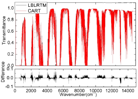
We have done many tests to reach the conclusion that the standard error between CART and LBLRTM is less than 3 %, Fig. 1 is an example of a comparison of CART with LBLRTM including molecular absorption, continuous absorption and scattering computed by using MT_CKD 1.2 method [9], the relative standard error is 1%.
At the mean time, we found CART is about 200 times faster than LBLRTM for using the fitting method. Thus, CART is a fast and more accurate transmittance model. This is the first feature of CART.
b) Feature 2: HITRAN 2004 database is used in LBLRTM calculation
HITRAN database is used in the LBLRTM calculation, however, HITRAN is a compilation of spectroscopic parameters and it has been updated seven times: HITRAN82 [10], HITRAN86 [11], HITRAN92 [12], HITRAN96 [13], HITRAN2k [14], HITRAN04 [15], ITRAN08 [16]. In order to provide and simulate the accurate transmission and radiation of light in the atmosphere, we should use the most accurate version of HITRAN.
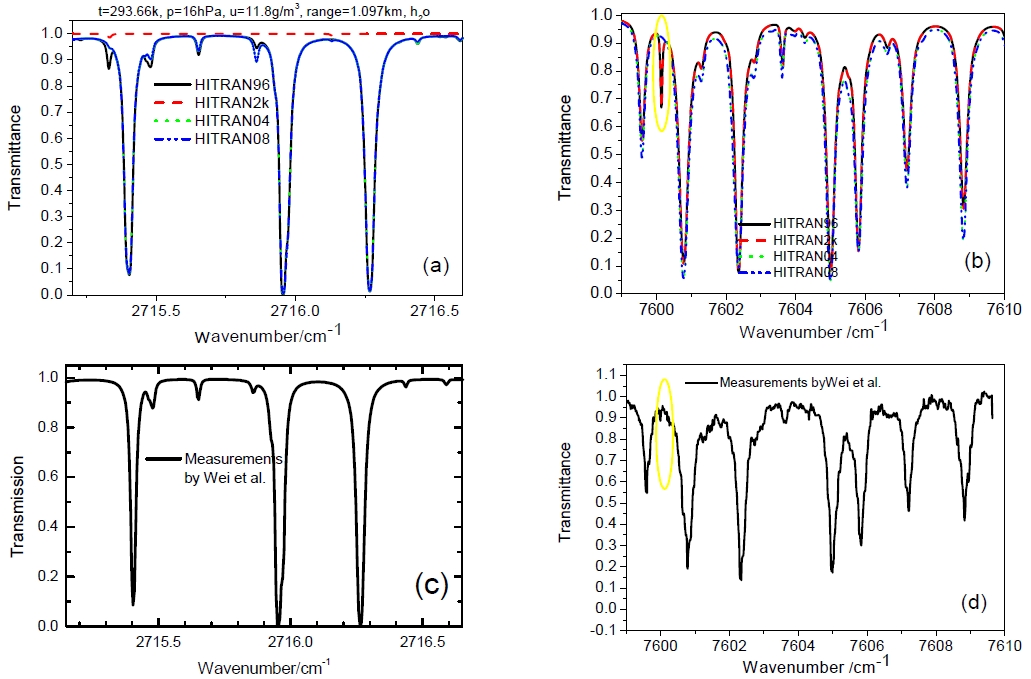
The transmittance calculations using HITRAN96, HITRAN2k, HITRAN04 and HITRAN08 over band1 (3.8 μm) and over band2 (1.315 μm) are compared, the results are shown in the upper two panels in Fig. 2. We found in the figure that there are three strong absorption lines in HITRAN96, HITRAN04 and HITRAN08, while no lines or very weak lines in HITRAN2k over band1; there is a strong line in HITRAN96 and HITRAN2k, but no line or very weak line in HITRAN04 and HITRAN08 at the spectral point of 7600.133 cm-1 circled in yellow in the right upper panel in Fig. 2; lines in HITRAN04 fit well with lines in HITRAN08. Which version of the HITRAN database is most accurate? We use some of the measured data to explain it as shown in the lower two panels in Fig. 2. The measurements by Wei et al. [17,18] showed that there are three strong absorption lines in the region from 2715 cm-1 to 2716 cm-1; but no strong absorption line at 7600.133 cm-1 was found. The result is consistent with HITRAN04 and HITRAN08. This illustrates that the strong absorption line at 7600.133 cm-1 does not exist, and shows that the HITRAN 96 and HITRAN 2k have some errors, while lines in HITRAN 04 and HITRAN 08 fit with the measured lines, so the calculated results will be more accurate in CART because the HITRAN 04 is used in it, HITRAN 08 is not used because it had not been released when the CART began development. This is the second feature of CART.
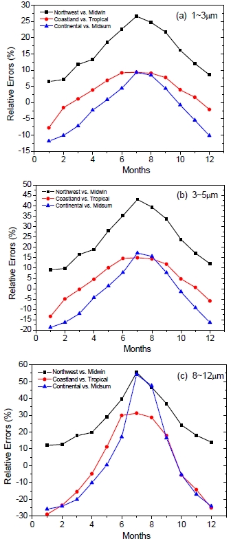
c) Feature 3: More atmospheric models in China are put into CART
The atmospheric environments of China are very complicated, the atmospheric models of China are absent in MODTRAN, LOWTRAN, FASCODE and LBLRTM, in which there are only six atmospheric models marked according to latitude. It will bring difference to simulate the transmittance or radiance in the regions of China by using the six standard atmospheric models.
We have collected 39 atmospheric models in three regions of China (northwest from Jan. to Dec. and yearly averaged, coastland from Jan. to Dec. and yearly averaged, and continental from Jan. to Dec. and yearly averaged). Northwest is a dry area with desert, Coastland is the area at the junction of ocean and land, while continental is a land area with medium humidity. We compared computed transmittances over three wavebands (1~3 μm, 3~5 μm and 8~12 μm) using the atmospheric models of China with results using the standard atmospheric models. The results are shown in Fig. 3. It shows that the maximum error between atmospheric models of China with a standard atmospheric model is up to 50%, the errors are different for different months and for different wavebands. Obviously, it will be more accurate to use the atmosphere model tailored for China for the calculation in regions of China. This is the third feature of CART.
d) Feature 4: An aerosol model based on measurement size distribution parameters is added
The transmittance of aerosols from
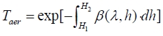
where β(λ,
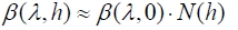
where β(λ,0) is the spectral distribution of aerosols at the surface
We add a model for aerosol extinction based on the real measured size distribution and profile of aerosol extinction coefficient at LIDAR wavelength. For a given size distribution d
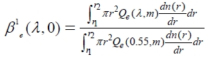
Where
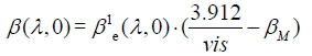
βM is the extinction of molecules at surface, and it is assumed to be 0.001159 km-1. The real
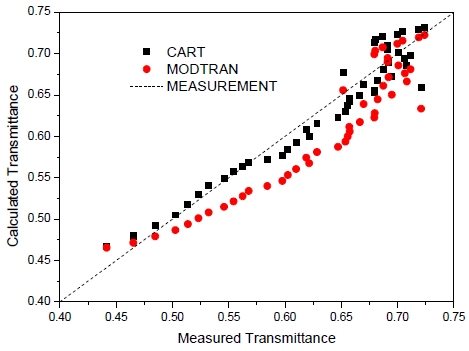
We have compared the calculated extinction using the above model in CART and calculated data using the MODTRAN model with the data measured by the grating sunphotometer (pgs100) which is manufactured by Prede Co. Ltd.. The size distribution of aerosol measured by Optical Particle Counter (OPC), and the height distribution of aerosol extinction measured by 532 nm MPL LIDAR are input parameters for CART, but MODTRAN uses the rural spectral aerosol model and Spring-Fall height distribution, the other parameters are the same. For example, the surface visibility is 11.3 km, and the relative humidity is 79%. Fig. 4 compares the results. We can see from the figure that the results computed by CART are closer to the measured data,
e) Feature 5: A fast multiple-scattering algorithm based on DISORT is adopted for radiance calculation over a broad waveband
The discrete ordinate radiative transfer (DISORT) [19] is a rigorous method for simulating the transfer of radiation in a vertically inhomogeneous, nonisothermal, plane-parallel medium. However, it is not computationally efficient to use DISORT for many applications. It is required that a fast and accurate radiative transfer model for multiple scattering should be developed.
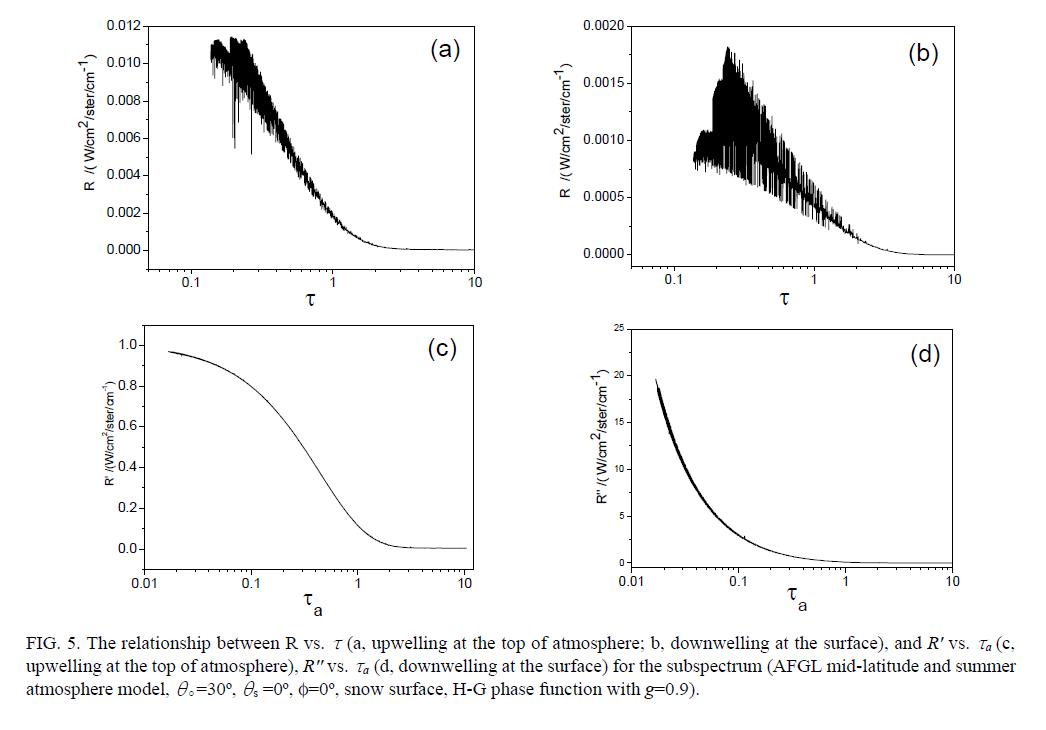
We compute the radiance and τ (total optical depth) in a subspectrum, then analysis the relationship between radiance and τ, see Fig. 5 (a) for upwelling at the top of atmosphere and (b) for downwelling at surface, H-G phase function (P=(1-g2)/(1+ g2-2g ?μ)3/2, g is asymmetric factor, μ is the cosine of scattering angle) is used. It shows that the radiances vary abruptly with τ, so, we make some changes. Because for the case of upward radiances at the top of atmosphere, it includes reflected radiance from the surface and earth emission, the radiances
The detailed treatments are as follow: Firstly, we divide the whole waveband into some subspectra; Secondly, for each subspectrum, the pre-computed τa obtained from CART are sorted in an ascending order; Next, seven uniformly logarithmic τa are selected, for each selected point, the radiances are computed using DISORT and converted to
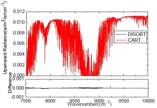
Fig. 6 is the comparison of upwelling radiances calculated using the fast model for multiple scattering in CART with directly calculated data using DISORT. It shows that results of the fast model agree well with the results of DISORT. We have done many tests to determine that, the relative errors between the fast model and DISORT are less than 2%, while, the computational efficiency is higher than that of DISORT by a factor of two orders. Thus, this method is fast and accurate, and this fast method can also be applied to a cloudy sky condition, which is the fifth feature in CART.
This section introduces the applications of CART for the simulations of atmospheric transmittance and background radiance.
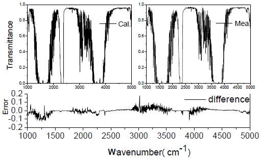
a) Application 1: Simulating the measured transmittance by FTIR (Fourier transform infrared) in atmosphere along a horizontal path
An atmospheric transmittance measuring system was set up to measure horizontal atmospheric spectral transmittance by using a standard blackbody with temperature of 1273.15 K as the light source, the blackbody light is transmitted parallel through a small diaphragm by an abaxial paraboloid collimator. The receptor of the system is an interferential Michelson in the FTIR which is at a distance (about 320 m) from the transmitter. The interference pattern is collected and converted to spectral intensity using a Fourier transform. Then the transmittance is obtained by comparing the calibrated spectral intensity and the transmitted spectral intensity. The FTIR uses two infrared detectors to achieve the wide spectral range (700-5000 cm-1), the MCT detector is for the spectrum from about 700 to 2000 cm-1, and the InSb detector for the part from about 2000 to 5000 cm-1, with spectral resolution of 1 cm-1.
The transmittance for the same condition is simulated by using CART. The atmospheric parameters for the CART simulation are measured synchronously by a surface measuring system at that time. A comparison of the results of simulated and measured transmittance are shown in the upper panels in Fig. 7, and the differences are shown in the lower panel. We found that the simulated data agree well with the measured data. In this spectral region, the relative error is 5.4%. The absorption by many molecules in the atmosphere occur in the region, for example, water vapor at 2.7 μm and 6.3 μm, carbon dioxide at 4.3 μm, ozone at 9.6 μm, and methane at 7.6 μm. With the accurate transmittance model, the types of molecules in the atmosphere can be retrieved from the measured data. This is the first application.
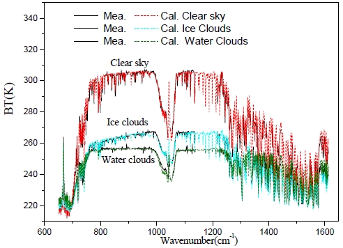
b) Application 2: Simulating the AIRS measured upwelling brightness temperature (BT)
We can demonstrate the performance of CART by simulating the spectral infrared radiance measured by AIRS (Atmospheric Infrared Sounder) [20] under both clear and cloudy conditions (both water and ice clouds). Singlelayered clouds are assumed to reside in a plane-parallel, homogeneous and isothermal layer in a given field of view (FOV). Bulk cloud single-scattering properties (SSP) are obtained from the parameterized coefficients of SSP of water clouds and ice clouds. The SSP of water clouds are calculated by using Mie code, and SSP of ice clouds are from Yang et al. 2000 [21] and Yang et al. 2005 [22].
An AIRS granule measured at 1917 UTC on September 6, 2002 is used for a case study. Three fields of view (FOVs) are chosen: clear sky, cirrus clouds, and optically thick water clouds. Optical thickness of clouds for three FOVs are 0.0, 0.85 and 5.8 respectively; the cloud heights of cirrus and water clouds are 9.0 km and 6.5 km respectively; and effective radius for ice and water clouds are 100.0 and 15.0 μm. The results between simulated upward BTs and AIRS observed data are shown in Fig. 8. From Fig.8, it is shown that the simulated results coincide well with the AIRS high spectral observations both for clear sky and cloudy conditions. The results illustrate that this fast model in CART can be used to fast simulate the moderate spectral resolution (including low spectral resolution) observations, such as the AIRS observed data, both for clear and cloudy sky conditions (ice clouds and thick water clouds). Because, there is much information included in the observed infrared data, including optical thickness of clouds, cloud effective radius and cloud height, the fast model in CART can be further applied for remote sensing of clouds. This is the second application of CART.
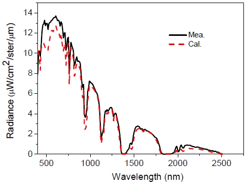
c) Application 3: Simulating the AVIRIS observed visible/ infrared upwelling spectral radiance
The Airborne Visible/Infrared Imaging Spectrometer (AVIRIS) [23] which is onboard the NASA ER2 aircraft flying at a height of about 20 km, measures the upwelling spectral radiance from the sun that was reflected by the surface as well as absorbed and scattered by the intervening atmosphere from 400 to 2500 nm through 224 contiguous spectral channels. These spectra are used to identify and determine the abundances of constituents of the Earth's surface and atmosphere through the analysis of spectral molecular absorptions and scattering properties of materials. Therefore, it is important to simulate the measured spectral radiances.
A case AVIRIS observed at 1852 UTC on June 23, 1997 is studied, which is a clear sky over Oakland (38.4° N,-116° E, land surface). The observing height is 20.2 km, the surface albedo is a function of wavenumber, the surface temperature is 294.88 k. The profiles of temperature, pressure, and relative humidity are obtained from a nearby Vaisala sonde. These parameters are input into CART to simulate the upwelling spectral radiance. The compared results of simulated and measured data are shown in Fig. 9. In the figure, the simulated data are scaled to 10 nm to match the spectral resolution of AVIRIS. The figure shows that the simulated data generally agree with the AVIRIS measured data, but the simulation and observation still have some difference especially at the visible wavelengths. This is because the spectral surface albedos do not match the real data in Oakland. So, the spectral surface albedos can be retrieved by applying CART to simulate the observed upwelling spectral radiance. This is the third application of CART.
We have investigated a combined atmospheric transfer model (CART), which is a set of fast and accurate models for calculating spectral transmittance, radiance (including scattered, thermal, and surface reflected). The spectral resolution is 1 cm-1, the spectral region extends from visible to far infrared wavelength.
Five features are described in detail in this paper to illustrate that CART differs from other models, and has some superiorities to those models. But there may be many insufficiencies which should be improved. The study of the combined atmospheric transfer model is a challenging and long-range work.
Three applications are also introduced: simulating the measured transmittance along a horizontal path, upwelling infrared brightness temperatures, upwelling visible/infrared spectral radiances. Of course, CART can be used to simulate other cases, like transmittance along slant paths, downwelling brightness temperatures or radiances. Furthermore, we will use CART for the retrieval of identities of atmospheric molecules, clouds and other information in the atmosphere.