A micro-pulse LIDAR system (MPL) was employed to measure the aerosol over Pudong, Shanghai from July 2008 to January 2009. Based on Fernald method, aerosol optical variables such as extinction coefficient were retrieved and analyzed. Results show that aerosol exists mainly in low layers; aerosol loading reaches its maximum in the afternoon, and then decreases with time until its minimum at night. Most of the aerosol concentrates in the layer below 3 km, and optical extinction coefficient in the layer below 2 km contributes 84.25% of that below 6 km. Two extinction coefficient peaks appear in the near surface layer up to 500 m and in the level around 1000 m. Aerosol extinction coefficient shows a seasonal downward trend from summer to winter.
Aerosol consists of solid or liquid particles floating in the atmosphere, with a diameter of 0.001~ 100 μm. It comes from two sources, natural or anthropogenic. Natural sources include volcano ashes, pollen, eroded rock particles, forest fire smoke and fine salts broken from sea foams by blowing wind. Anthropogenic sources include smoke from burning biosmass and industrial releases. Aerosol plays a very important role in atmospheric environment and climate change, though it is only a trace substance in the atmosphere.
Data like visibility [1, 2], surface solar radiation[3-5], sun-photometer and satellite measurements[6-9] can be used to study aerosol distribution features and its impacts. For example, by analyzing remote sensed MODIS (Moderate Resolution Imaging Spectroradiometer) data, Duan[10] found that the area of high aerosol optical depth over Changjiang Delta, eastern China, tends to increase annually. A LIDAR not only can measure aerosol in real time, but also can provide aerosol vertical distribution, therefore, LIDAR is an effective device for aerosol research. Lu[11] quantitatively measured and processed data for the aerosol over Beijing using sunlight attenuation and LIDAR measurement. Zhou[12] used both L625(laser wavelength is 0.635 μm) and L300 (laser wavelength is 0.3 μm) LIDARs to observe aerosol, and found seasonal variations of mixing layer, boundary layer, and aerosol distribution. According to LIDAR measurements over Beijing and Naqu, Tibet, Liu[13] got and analyzed the vertical distribution of aerosol extinction coefficients. With a Nd:YAG LIDAR system, Chiang[14] measured the aerosol over Chung-Li, Taiwan, and found that 40%~50% of the aerosol total extinction coefficient was contributed by the aerosol in the 1~5 km low layer.
A new type micro-pulse LIDAR (MPL) produced by SigmaSpace was mounted in Pudong, Shanghai, and started to work on July 1, 2008. With the LIDAR measurement, aerosol properties over Pudong, Shanghai are analyzed.
Shanghai is one of the largest cities China. It sits on the Yangtze River Delta on China's east coast, with a humid subtropical climate and four distinct seasons. It is generally sunny in spring and autumn, has plenty of rain and the average number of rainy days is 112 per year. In Pudong, Shanghai, great amounts of anthropogenic aerosol are produced by automobiles and industrial release, but rainfall cleaning and deposition decrease aerosol loading. So it is interesting to track the variation of aerosol. However, this paper focuses on the statistical features of aerosol based on LIDAR measurement.
The SigmaSpace-made micro-pulse LIDAR has advantages for aerosol measurement. Main parameters of the LIDAR are listed in table 1. The green light emitted by the LIDAR has a wavelength of 527nm. Pulse repetition frequency is 2500 Hz. Bin time is 100ns, 200ns and 500ns, which means the LIDAR data has a vertical range resolution of 15m, 30m and 75m. Data integral time is 30s, which implies that every record data comes from the echo average over 75000 pulses (2500 × 30 = 75000). Under clear weather, the maximum detectable height is about 20 km (60 km theoretically) in nighttime, but only 10km in daytime.
Many factors such as background noise will influence the LIDAR measurement and data quality, so the echo data should be processed before retrieving aerosol variables. The pre-processing includes detector delay correction, background noise correction, parasitic pulse correction, geometric factor correction and range correction [15,16]. The LIDAR receiver picks up the backscattered laser energy from aerosol particles within a sampling volume. The echo power and aerosol variables are dominated by following equation (LIDAR equation):
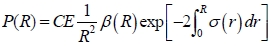
Where, P(R) is the received backscattered power, C is the system constant, E is transmitted pulse power, β(R) is backscattered coefficient, σ(r) is extinction coefficient. In the equation, the received power P(R) is known, C and E are provided by manufacturer, but β(R) and σ(r) are unknown. So the equation is hard to solve. Generally, β(R) and σ(r) are dominated by both aerosol and gas molecules, i.e.,
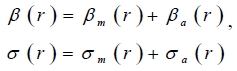
In order to retrieve aerosol information, both β(R) and σ(r), or one of them must be solved from the equation. With the relationship bridged between β(R) and σ(r), the equation can be solved.
[TABLE 1] Main parameter of the MPL
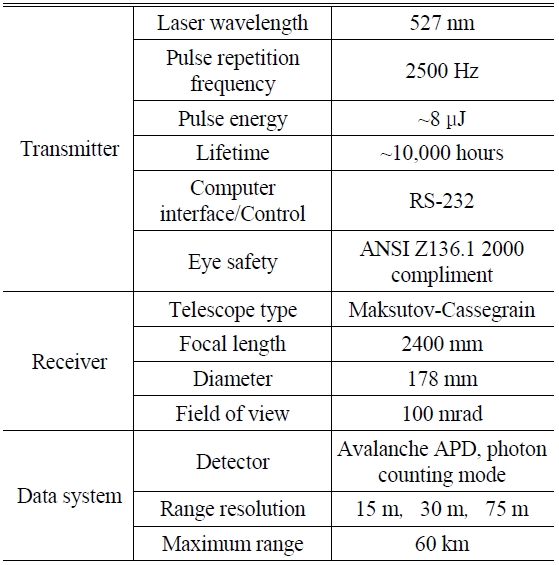
Main parameter of the MPL
Fernald retrieval method [17] is adopted here to extract aerosol extinction coefficient from LIDAR measurement. To retrieve the aerosol extinction coefficient in the layer below 6 km, the reference height rc is chosen as 3~5 km according to Zhou[12]. Taken into account the release from the great amount of automobiles and factories in Shanghai, the ratio of aerosol extinction coefficient to backscattered coefficient is assumed to be 30[14], i.e.,
.and the aerosol backscattered ratio is assumed to be 1.05, i.e.,
Where, subscript
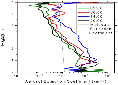
To analyze the diurnal variation of aerosol, LIDAR measurements at 02:00,08:00,14:00 and 20:00BST (Beijing Standard Time) are used for processing. First, pick up the four-time data of each clear day(without obvious cloud below 6 km), make average over 15 minutes, then adopt Fernald method for retrieval. Afterwards, daily variables are obtained by averaging the 4 time retrievals.
3.1. Diurnal variation of aerosol extinction coefficient
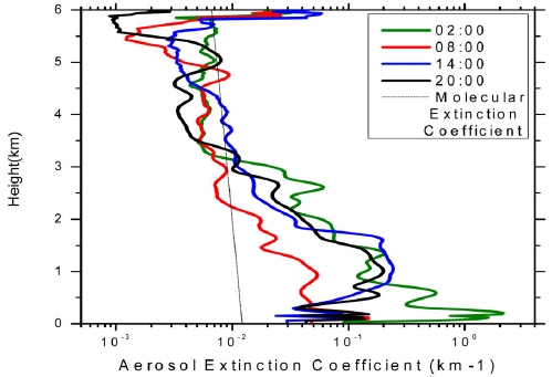
The diurnal variation of aerosol extinction coefficient in July 2008 is shown in fig. 1. It can be seen that a small coefficient in morning (08:00) increases with time until afternoon (14:00).Then, it decreases with time until night (02:00), reaching its minimum. Such a variation may be dominated by the solar heating in daytime and radiation cooling at nighttime. Solar heating causes surface and low layer temperature rise, lifting up the aerosol to higher level. Radiation cooling at night strengthens aerosol deposition. Aerosol deposition and anthropogenic release from the ground surface are probably the reasons why an extinction coefficient maximum appears in surface layer below 500 m. From the middle of the night to morning, most aerosols lie in a low layer below 1 km. A similar aerosol vertical distribution appears in August, September, November, December and January, but the extinction coefficient in the October night is little bit bigger (Fig. 2), the reasons await further analysis and explanation. One possible reason is the biomass burning from countryside because october is the harvest month in Shanghai area. Farmers often burn dried plant in the evening. However, the near surface (below 200m) data is not very reliable, because the impact of LIDAR blind zone and geometric factor correction.
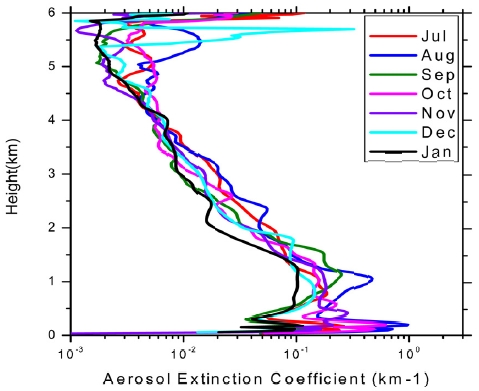
3.2. Monthly variation of aerosol extinction coefficient
The extinction coefficient gradually decreases with altitude, shown in Fig. 3. Such a variation appears in all months from July 2008 to January 2009. However, high extinction coefficient around 6 km may impacted by cloud (stratus), so the layer discussed in this section is confined below 4 km to avoid cloud influence. In low layer, especially below 2km, the extinction coefficient decreases with season from summer to winter due to weakened convection. Above the 3 km level, the extinction coefficient does not vary significantly in these months because of relatively homogeneous weather conditions. But two extinction coefficient peaks always exist in the layers below 500m and around 1000m. These peaks also appear in Fig. 1 and Fig. 2. The peak below 500m is caused by human activity releases and the dust which is forced up from the street and ground by convection and wind blowing. The released giant aerosol particles can not rise to higher layers, and they easily to sink down to the surface, and the fine particles may rise up to a higher level. Due to the impact of so many high buildings, the released giant and big aerosol particles can't rise to high layer and easy to sink down to surface, causing a extinction coefficient peak below 500m. The peak around 1000m is caused by local convection and aerosol long range transport from western and northwest industrial regions. Fine aerosol particles from industrial cities Suzhou (about 100 km west), Wuxi (about 150 km) and Changzhou (about 200 km) etc. can be driven over long range by a northwest wind to Shanghai. Such a transport is probably the main reason why an extinction coefficient peak exists around 1000m over Shanghai.
3.3. Vertically variation of aerosol extinction coefficient
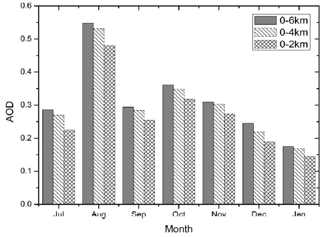
To analyze the vertical variation of the aerosol extinction coefficient, data from MPL is first retrieved and converted into extinction coefficients by adopting Fernald method, then, aerosol optical depth (AOD) is obtained by integrating the coefficient with height. In Fig. 4, AOD6 refers to the AOD of layer within 0~6 km, AOD4 means the AOD of layer 0~4 km, and AOD2 is the AOD of layer 0~2km. From Fig. 4, it is found about 84.52% of AOD6 is contributed by AOD2, which means most aerosol floats in the low layer of the atmosphere. This reflects that human activity and release is the main source of low layer aerosol.
3.4. Seasonal variation of aerosol
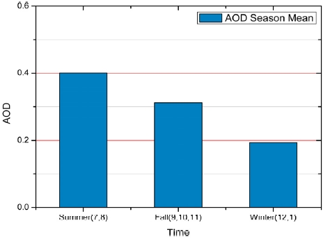
Only 3 season datasets were analyzed due to the lack of MPL measurement in spring and early summer. The seasonal averaged AOD in Fig. 5 was originally obtained by integrating the extinction coefficient with height up to 4 km. Fig. 5 shows, summer AOD is 0.4007, autumn AOD is 0.319 and winter AOD is 0.1936. The data implies Shanghai has a clear atmosphere in winter, but in summer, a little bit turbid. Perhaps the rich vapor contributes to AOD in summer, but how much is water vapor contribution is still unknown to us.
Aerosol optical property variables were analyzed based on MPL measurements in Pudong, Shanghai from July 2008 to January 2009. Main results are: (1)Aerosol extinction coefficient reaches its maximum at 14:00, then decreases with time and reaches its minimum at 02:00. Such a variation is relevant to solar heating in daytime and radiation cooling in nighttime. (2) From July to January, the monthly averaged aerosol extinction coefficient below 2 km level decreases gradually. Above 3 km, the monthly averaged extinction coefficient does not change significantly. In the surface layer below 500 m and the level around 1000 m, there remain two extinction coefficient peaks, caused mainly by local human activity and long range transport respectively. (3) AOD of layer below 6 km is mostly contributed by AOD below 2 km because AOD2 contributes 84.25% of AOD6.