In this study, the response surface method and experimental design were applied as an alternative to conventional methods for the optimization of coagulation tests. A central composite design, with 4 axial points, 4 factorial points and 5 replicates at the center point were used to build a model for predicting and optimizing the coagulation process. Mathematical model equations were derived by computer simulation programming with a least squares method using the Minitab 15 software. In these equations, the removal efficiencies of turbidity and total organic carbon (TOC) were expressed as second-order functions of two factors, such as alum dose and coagulation pH. Statistical checks (ANOVA table, <italic>R</italic>2and <italic>R</italic>2adjvalue, model lack of fit test, and p value) indicated that the model was adequate for representing the experimental data. The p values showed that the quadratic effects of alum dose and coagulation pH were highly significant. In other words, these two factors had an important impact on the turbidity and TOC of treated water. To gain a better understanding of the two variables for optimal coagulation performance, the model was presented as both 3-D response surface and 2-D contour graphs. As a compromise for the simultaneously removal of maximum amounts of 92.5% turbidity and 39.5% TOC, the optimum conditions were found with 44 mg/L alum at pH 7.6. The predicted response from the model showed close agreement with the experimental data (<italic>R</italic><sup>2</sup>values of 90.63% and 91.43% for turbidity removal and TOC removal, respectively), which demonstrates the effectiveness of this approach in achieving good predictions, while minimizing the number of experiments required.
Coagulation has been widely investigated for the removal of turbidity and natural organic matter (NOM) in water treatment. The effectiveness of coagulation influences the efficiency of subsequent sedimentation and filtration processes in water treatment [1]. The performance of coagulation is affected by many factors, not only the characteristics of raw water, such as the amount of particulate material, the amount and nature of NOM present and the chemical/physical properties, but also the conditions of coagulation, such as coagulant type, dose, and pH [2].
For individual water, the performance of a coagulant depends on two effective factors; the coagulant dose and coagulation pH. To seek the optimal conditions for these factors, jar tests using a conventional multifactor method, also known as one factor at a time (OFAT) method, was employed. In this approach, optimization is usually carried out by varying a single factor, while keeping all other factors fixed at a specific set of conditions. The OFAT method is not only time and energy consuming, but also usually incapable of reaching the true optimal conditions because it ignores their interactions [3]. On the other hand, the statistical method using response surface methodology (RSM) has been proposed to determine the influences of individual factors and the influence of their interactions. RSM is a technique for designing experiments, building models, evaluating the effects of several factors, and achieving the optimum conditions for desirable responses with a limited number of planned experiments [4]. RSM helps to demonstrate how a particular response is affected by a given set of input variables over some specified region of interest, and what input values will yield a maximum (or minimum) for a specific response. RSM was initially developed for the purpose of determining optimum operation conditions in the chemical industry, but it is now used in a variety of fields and applications, not only in the physical and engineering sciences, but also in biological, clinical, and social sciences [5]. The response surface design was used in this study to: 1) find how jar tests comprising of several levels of coagulation factors can be simplified, 2) determine how turbidity and total organic carbon (TOC) (as responses) are affected by changes in the level of alum dose and coagulation pH (as factors), 3) determine the optimum combination of dose and pH that yields the best removal of turbidity and TOC, and 4) quantitatively measure the significance and interaction between factors with respect to the optimum turbidity and TOC removals.
In this study, synthetic water was used as a raw water to maintain a consistent water quality while conducting the experiments. Commercial humic acid and kaolin (Sigma Aldrich, Milwaukee, WI, USA) were used to simulate humic substances and particles in surface water. The synthetic water was prepared by mixing prescribed amounts of kaoline clay and stock solution of humic acid in tap water. The humic stock solution was made by dissolving 1.5 g humic acid in 1,000 mL of 0.01 M NaOH with 6 hours continuous stirring, filtered through 0.45 μm membrane filter and stored in refrigerator for later use. The characteristics of the synthetic water are given in Table 1.
[Table 1.] Characteristics of the synthetic water [6]
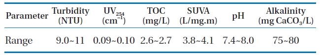
Characteristics of the synthetic water [6]
Alum was used as a coagulant in this work. The alum was in the powder form, with the formula: Al2(SO4)3.16H2O, and supplied by Sigma. The coagulation pH was adjusted using 0.1 M HCl or 0.1 M NaOH just before dosing of the coagulant.
When process factors (independent variables) satisfy an important assumption that they are measurable, continuous, and controllable by experiments, with negligible errors, the RSM procedure was carried out as follows:
A series of experiments were performed for adequate and reliable measurement of the response of interest.
A mathematical model of the second-order response surface with the best fit was developed.
The optimal set of experimental parameters producing the optimum response value was determined.
The direct and interactive effects of the process parameters (factors) were represented through two and three-dimensional plots.
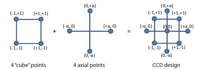
The first requirement of the RSM, as mentioned above, involves the design of experiments to achieve adequate and reliable measurements of the response of interest. A central composite design (CCD), which is a very efficient design tool for fitting second-order models [7], was selected for use in this study. The number of tests required for a CCD include: the standard 2
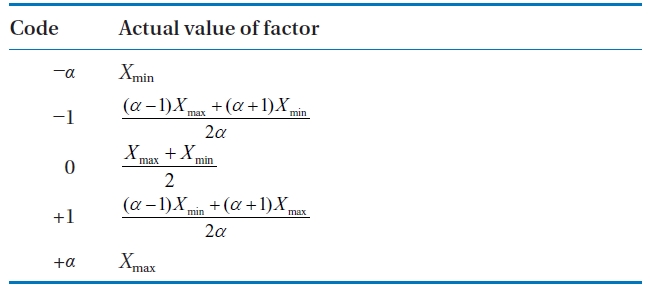
In order to define the experimental domain explored, preliminary experiments were carried out to determine narrower, more effective ranges of alum dose and pH prior to designing the experimental runs. It was found from the preliminary tests that coagulation was most effective in the range of alum doses from 12 to 68 mg/L and pH in the range from 5.5 to 8.5. Once the desired value ranges of the variables had been defined, they were coded to lie at ±1 for the factorial points, 0 for the center points, and ±αfor the axial points. The codes were calculated as functions of the range of interest of each factor, as shown in Table 2. A CCD with 4 factorial points, 4 axial points and 5 additional experimental trials (run numbers 10~13) as replicates of the center point are given in Table 3.
[Table 2.] Relationship between the coded and actual values of a factor

Relationship between the coded and actual values of a factor
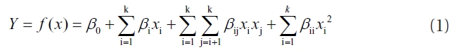
where
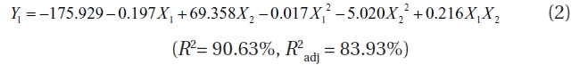
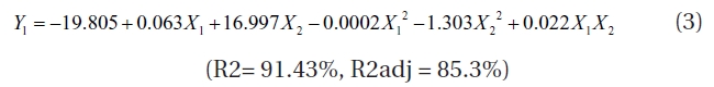
thirteen observed responses were used to compute the model using the least square method. The two responses (% turbidity and TOC removal) were correlated with the two factors (alum dose and coagulation pH), using the second-order polynomial, as represented by Eq. (1). From the experimental data, quadratic regression models were obtained, as shown in Eqs. (2) and (3):
Turbidity removal (%):
[Table 3.] CCD and the results obtained
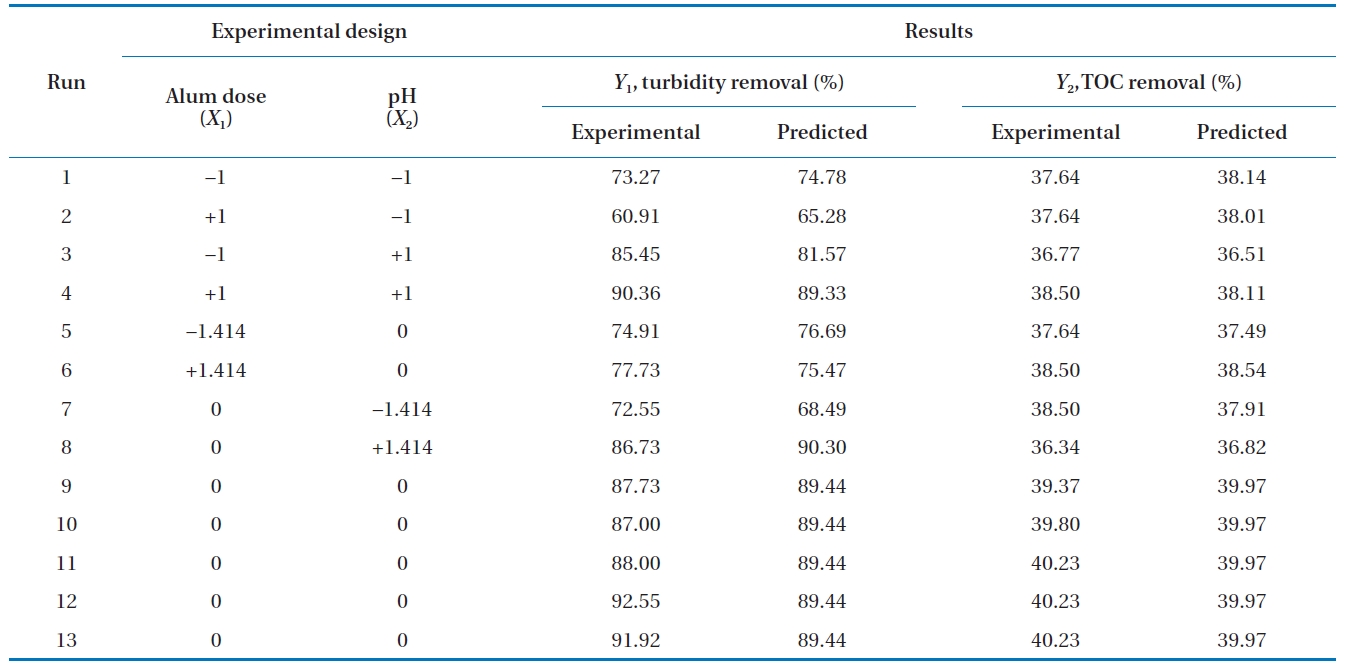
CCD and the results obtained
TOC removal (%):
where
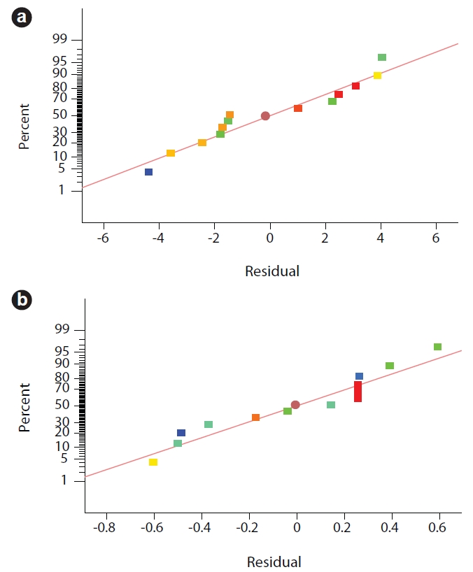
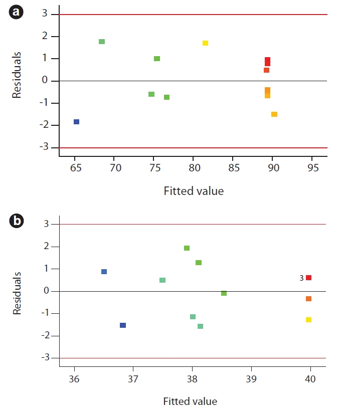
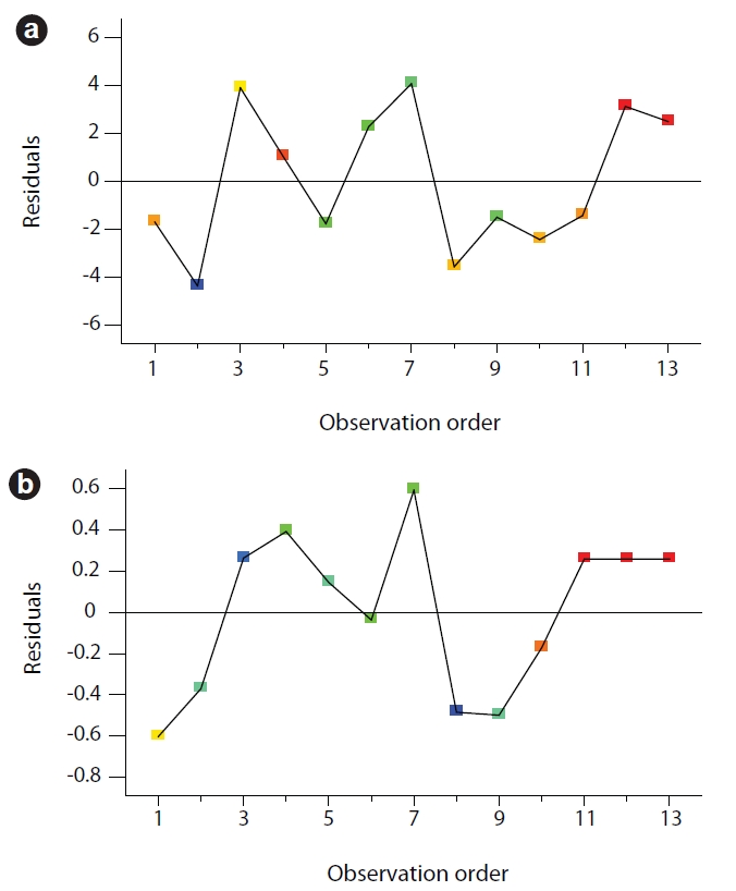
It is usually necessary to check the fitted model to ensure it provides an adequate approximation to the real system. Unless the model shows an adequate fit, proceeding with investigation and optimization of the fitted response surface is likely to give poor or misleading results. Graphical and numerical methods, as a primary tool and confirmation for graphical techniques were used to validate the models in this study [9]. The graphical method characterizes the nature of residuals of the models. A residual is defined as the difference between an observed value
The models were then checked using a numerical method employing the coefficient of determination (
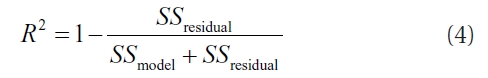
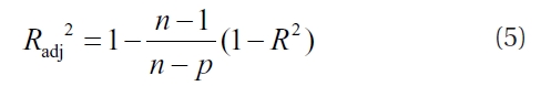
where SS is the sum of the squares,
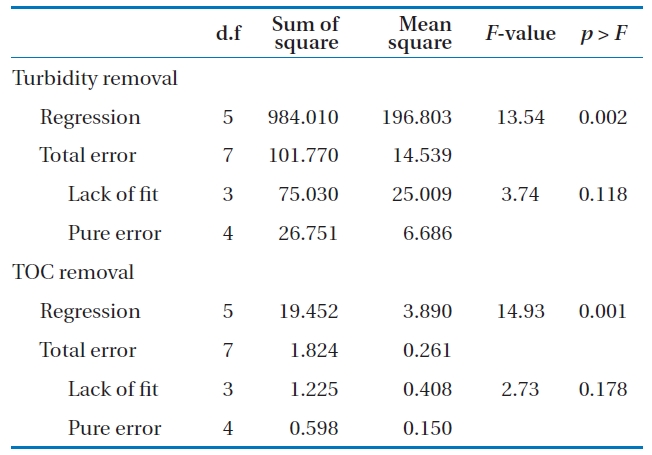
The ANOVA in Table 4 also shows the results of the lack of fit test for the models. The lack of fit test describes the variation in the data around the fitted model. If the model does not fit the data well, the lack of fit will be significant. The large
[Table 4.] ANOVA results for the two responses: turbidity removal and TOC removal

ANOVA results for the two responses: turbidity removal and TOC removal
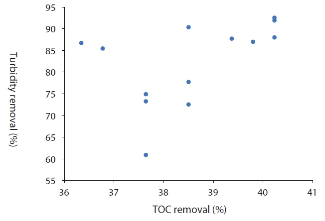
Fig. 5 shows the plot of turbidity removal vs. TOC removal data from the coagulation test. As shown in Fig. 5, no clear correlation between these two responses is noted. Therefore, the removal mechanisms of turbidity and TOC were different and the optimum conditions for the removal of each substance would also be different.
The results in Table 5 also indicate that pH (quadratic) was the most significant factor in determining the optimum TOC removal, with
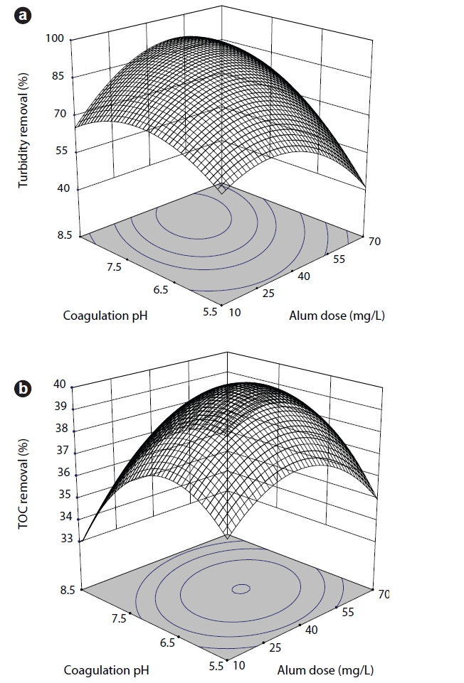
Except for the pH with respect to turbidity removal, the linear effects of pH and dose were insignificant/less significant in the statistical analyses, and became highly significant only by the quadratic effects. This difference implies that the models were not influenced by dose and pH in a linear manner, but strongly influenced by these factors in a quadratic manner. This trend can be observed in Fig. 6, with both curves showing very prominent changes. Although their linear effects were insignificant, the impacts of pH and dose to the coagulation process were still significant due to the quadratic effects towards turbidity and TOC removals. The roles of the coagulant dose and pH in coagulation are also underlined in other studies [2, 11].
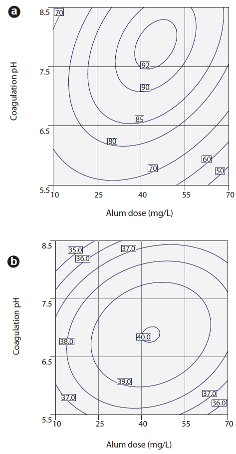
Figs. 6 and 7 show the 3-D surface and 2-D contour plots, respectively. The response surface and contour plots are the graphical representation of the regression equation used to visualize the relationship between the response and experimental levels of each factor. As shown in these plots, increased turbidity removal was observed with increasing alum dose and pH values. However, an increase in both factors beyond the optimum region resulted in a decrease in the removal efficiency. At alum doses higher than 50 mg/L, the turbidity removal began to decrease at all of coagulation pHs, implying re-stabilization of the particles due to overdosing. With respect to TOC removal as a response, an increase in the removal efficiency was observed with decreasing of pH. The plots also showed that higher pH values were favorable for coagulation of turbidity, while lower pH values improved the coagulation of TOC.
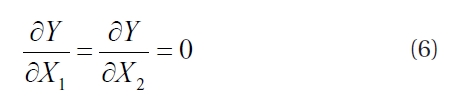
An optimum level of these factors was obtained by analyzing the response surface-contour and the derivative of Eqs. (2) and (3). The optimum conditions were a set of
The obvious prominence in the response surfaces indicated that the optimal conditions were located exactly inside the design boundary. The maximum predicted value was indicated by the surface confined in the smallest ellipse in the contour diagram. Moreover, a canonical analysis [7] of the two models resulted in Eigenvalues of λ1and λ2, which were both negative, such as λ1= -5.022 and λ2= -0.015 in the case of turbidity removal, and λ1= -1.30 and λ2= -0.002 for TOC removal, indicating that the stationary point was a single point of maximum response. The model predicted a maximum of 92.2% turbidity removal with an alum dose of 44 mg/L and pH 7.85, while the highest TOC removal was obtained under conditions of 44 mg/L alum and pH 6.90.
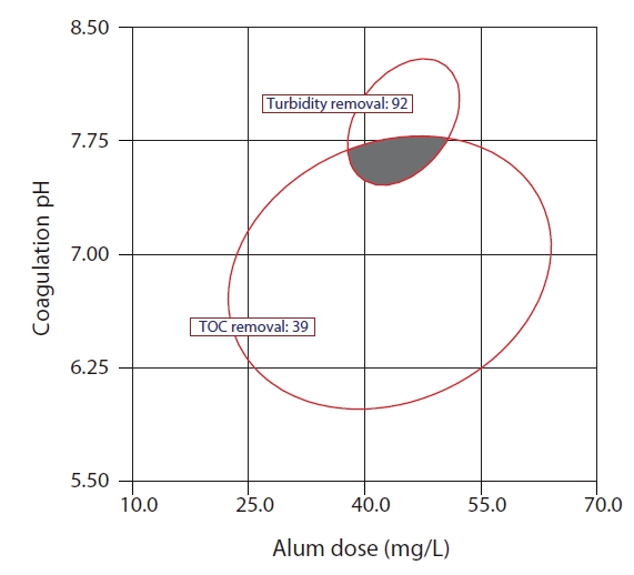
The turbidity and TOC removals were the two individual responses, and their optimizations were achieved under different optimal conditions. The optimum turbidity removal might aggravate TOC removal and vice versa [12]. Thus, a compromise between the conditions for the two responses is desirable. The optimum conditions for the simultaneous removals of turbidity and TOC can be visualized graphically by superimposing the contours for various response surfaces in an overlay plot. By defining the limits of the desired turbidity and TOC removals, the stripe portion of the overlain plot, as shown in Fig. 8, defines the permissible factor values. Base on the overlain contour, a compromise for 92.0% turbidity removal and 39.5% TOC removal can be met at 44 mg/L alum and pH 7.6.
[Table 5.] Estimation of the second-order response surface parameters (coded unit)
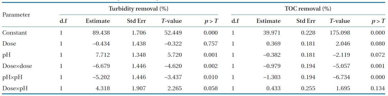
Estimation of the second-order response surface parameters (coded unit)
[Table 6.] Confirmation experiments at optimum conditions
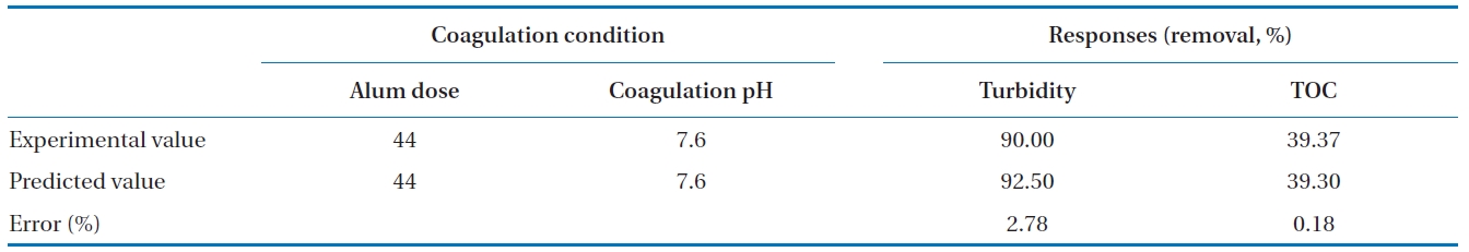
Confirmation experiments at optimum conditions
To confirm the agreements of the results achieved from the model and experiments, two additional experiments were conducted by applying the alum dose and pH in the optimum region. As shown in Table 6, the turbidity and TOC removals obtained from the additional experiments are very close to those estimated using the model, implying that the RSM approach was appropriate for optimizing the conditions of the coagulation process.
This work has demonstrated the application of RSM in seeking optimal conditions for coagulation tests. Simultaneous removals of turbidity and TOC were investigated. In order to gain a better understanding of the two factors for optimal coagulation performance, the models were presented as 3-D response surface and 2-D contour graphs. The following conclusions were obtained:
From the statistical analyses, the coagulant dose and coagulation pH have significant effects on the coagulation of turbidity and TOC.
A maximum amount of turbidity was removed using 44 mg/L alum at pH 7.8. At the same alum dose of 44 mg/L, reducing the pH to 6.9 resulted in maximum removal of TOC.
To simultaneously remove 92.5% turbidity and 39.5% TOC, 44 mg/L alum and pH 7.6 were selected based on the overlain contour.
The results of a confirmation experiment were found to be in good agreement with the values predicted by the model. This demonstrates that to obtain a maximum amount of information in a short period of time, with the least number of experiments, RSM and CCD can be successfully applied for modeling and optimizing the coagulation process.
This work was supported by the Pukyong National University Research Fund in 2008 (PK-2008-055).

![Characteristics of the synthetic water [6]](http://oak.go.kr/repository/journal/10074/E1HGBK_2010_v15n2_63_t001.jpg)