


A review of stormwater quality and quantity in the urban environment is presented. The review is presented in three parts. The first part reviewed the mathematical methods used in stromwater quantity modelling. This second part reviews the mathematical techiques used in stromwater quality modelling and has been undertaken by examining a number of models that are in current use.
2. Urban Runoff Quantity Problems and Models
2.1. Pollutant Build-up and Wash-off Model
2.1.1. Regression Model
Tasker and Driver (1988) developed simple regression model on the basis of long term urban runoff data and made it applicable for the unmonitored watershed based on some physical (drainage area, impervious percentage, percentage residential or/and industrial) and climatological data (total rainfall, storm duration, mean annual rainfall).1) The model uses the following generalized regression formula for calculating loads:
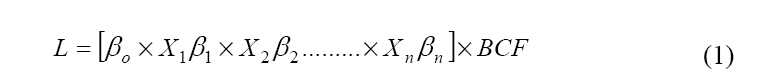
where,
The model parameters are estimated by a generalized-leastsquare regression method that accounts for cross correlation and differences in reliability of sample estimates between sites. The regression models account for 20 to 65 percent of the total variation in observed loads.
2.1.2. Simple Empirical Model
Schueler (1987) introduced an easy empirical equation based model known as Simplified Urban Nutrient Output Model (SUNOM) for urban pollutants load prediction based on five years data collected by United States Environmental Protection Agency (USEPA). The method uses the flow-weighted mean concentration. 2) The generalized equation is as follows:
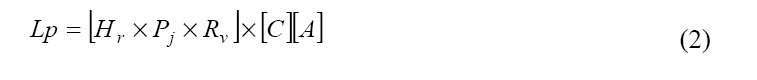
where
According to Schueler, the simple method does not consider base flow runoff and associated pollutant loads, and is better used at small watersheds. The model is rarely appered in the literature. Recently, the model was applied by Flint (2004) to estimate water quality an ultra urban area in Maryland, US.3)
2.1.3. Sartor and Boyd Model
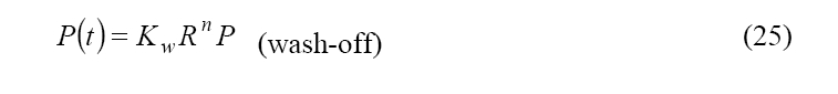
James Sartor and Gail Boyd first introduced this model in 1972 (Sartor and Boyd, 1972).4) This model provides the knowledge of pollutants transport and their quantification. The model shows the dislodging of the particles during a rainfall event is dependent on the street characteristics, rainfall intensity and the particle sizes where the wash off can be described by the following equation:
where,
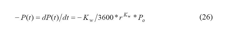
Many models such as PSRM-QUAL are based on equation 26 (PSRM-QUAL Users Manual, 1996) and kinematic wave equations.5) Once the particle is dislodged the shear forces generated by the runoff cause its movement when the runoff is above the critical velocity (velocity at which drage force and resistance forces are equal). Critical velocity is given by

where
where,
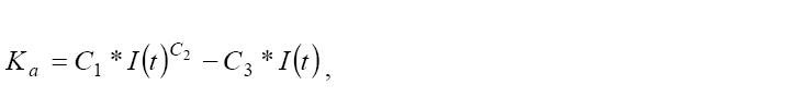
Haiping and Yamada (1996) applied Sartor and Boyd equation with refinement by adding some constants such as i) maximum amount of constituents on impervious areas (
where,
where,
Furumai et al., (2003) applied Sartor and Boyd model with some modification in urban catchment in Japan. They assumed that the runoff from road and roof are different so that the washoff behavior as follows.8) They provided two different runoff coefficients for road and roof.
where,
The above model (Furumai et al., 2003) was applied by Murakami et al., (2004) to predict the wash-off behavior of particlebound PAHs from road and roof and stated that the model could explain suspended solids and particle-bound PAHs runoff well except during and after heavy rainfall (>;10mm/hr).
Aryal (2003) applied Sartor and Boyd model to predict the pollutants wash-off behavior in highway runoff. As this equation states that the quantity of the constituents available for washoff decreases exponentially with runoff volume during the event, the model could not be applied to the events where the two or more pollutants loading pattern were observed due to the change in rainfall intensity (intermittent rainfall) during wet weather period.9) The Sartor and Boyd model found not suitable to the events where two or more SS loading patterns observed. This indicated difficulty in applying the model in those runoff events where the rapid fluctuation of concentration occurred. The following equation establishes the relationship between concentration and the Sartor and Boyd model.
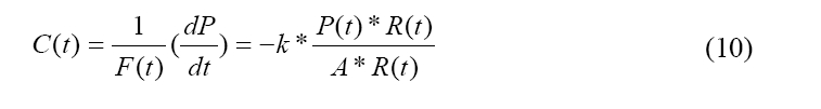

where,
This equation (11) shows that the primary difficulty of the Sartor and Boyd equation is that it always produces decreasing concentrations as a function of time regardless of the time distribution of runoff. This is counter-intuitive, since it is expected that high runoff rates during the middle of the storm might produce higher concentration than those proceeding. Aryal (2003) descretized the storm event and applied the model which he finally summed up to calculate the pollutant load.
Egodawatta et al., (2007) also applied the modified version of Sartor and Boyd model by introducing the capacity factor (CF). They reported that a storm event has the capacity to washoff only a fraction of pollutants available and this fraction varies primarily with rainfall intensity, kinetic energy of rainfall and characteristics of the pollutants. They then modified the Sartor and Boyd equation in order to incorporate the wash-off capacity of rainfall by introducing the ‘capacity factor’ CF. According to them, the fraction wash-off can be written as
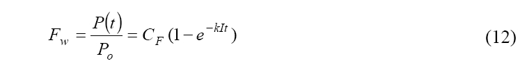
where, CF is the value ranging from 0 to 1 depending on the rainfall intensity. Other factors such as road surface condition, characteristics of the available pollutants and slope of the road may also have influence on CF.
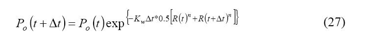
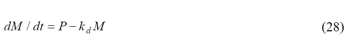
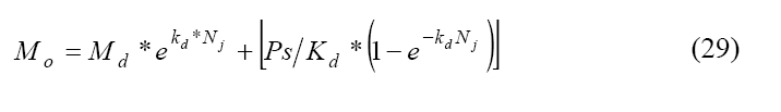
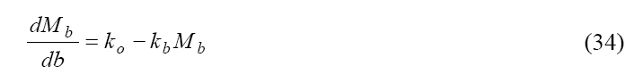
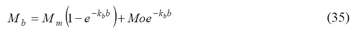
Chen and Adams (2007) also applied the Sartor and Boyd wash-off with refinement by introducing the pollutants accumulation rate based on Osuch-Pajdzinksa and Zawilski (1998) that can accommodate the dry weather period also.10,11) The rate of pollutant accumulation is:
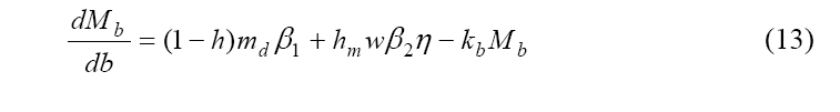
where
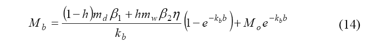
where, Mo is residual pollutant mass not washed off by the previous runoff event.
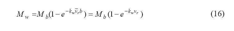
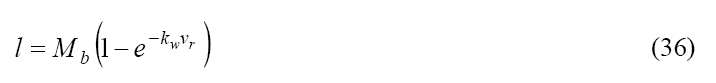
In their study they assumed that the rate of pollutant washoff from the catchment surface is proportional to the amount of pollutant build-up on the catchment surface and is directly related to the volume of runoff.
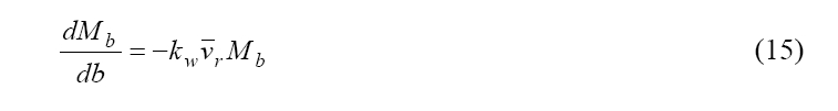
where r v is the average runoff rate in mm/hr,
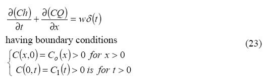
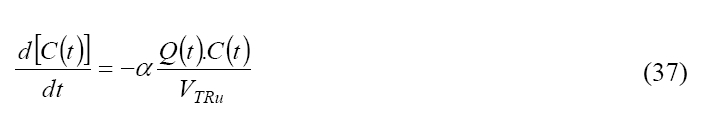
2.2. Advective Diffusion Model (Mass Transport Equation)
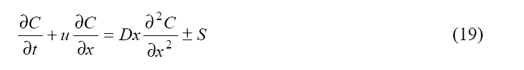
It is the one dimensional conservative advective-diffusion equation, that incorporates the advection and diffusion process is to describe the behaviour of a pollutant in stream;
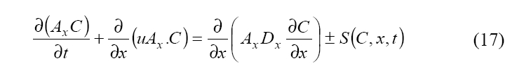
where,
This equation includes the advection of pollutants by the flowing water, diffusion of pollutants in the stream, constituent reactions, interactions and sources and sinks. Assuming that
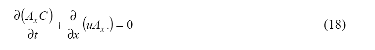
Then
which is the form of the advective-diffusion equation used in model like HEC-5Q and WQRRS.
Shaw et al., (2006) proposed a new stochastic physical model that is primarily focused on the rain flow transportation.12) The model was mainly based on Hairsine and Rose (1991) which states that the flow does not exceed the threshold for particles entrainment, mass conservation of suspended particles in the water layer:
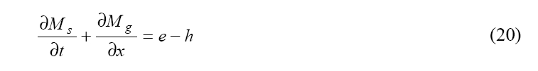
where,
Particles mass on the surface,
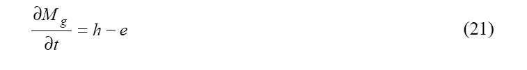
The value e was defined by
where,
They also applied water balance at a pint x by using the equation
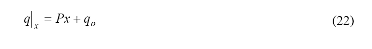
where, P is the rain intensity per unit width (mL min-1 cm-1), q is the flow reate per unit width (mL min-1 cm-1) and qo (mL min-1 cm-1) is the constant upslope inflow per unit width.
2.3. Kinematic Wave Equation Model
It is another governing one-dimensional equation for pollutant transport on a unit width basis, where solute is injected instantaneously, can be written as
where,
Qs = CQ
2.4. Other Stormwater Quality Models
2.4.1. SWMM
SWMM is one of the most successful model produced by United States Environmental Protection Agency (US-EPA). This model is not exclusively designed for urban drainage and single-event or long term (continuous) simulation. The earlier SWMM model used the linear build up formulation. The model provides three options for pollutant build up as follows:
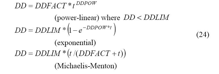
Among the above equation, exponential and Michaelis-Menton functions clearly define asymptotes or upper limits. Upper limits for linear or power function build-up may be imposed if desired. The wash-off equation as follows: using an exponential washoff equation as follows:
where,
As mentioned above earlier, primary difficulty in this equation is always producing decreasing concentrations as a function of time regardless of the time distribution of runoff (Aryal et al., 2003). This problem is overcome in SWMM by making washoff at each time step,
where,
It may be seen that if equation is divided by runoff rate to obtain concentration, then concentration is now proportional to ?rKw-1. Hence, if the increase in runoff rate is sufficient, concentrations can increase during the middle of a storm even if PSHED is diminished.
From the basic equation (48), the wash-off parameters, washoff coefficient and exponent are determined from a finite difference approximation (Nix, 1994) which produces:13)
where,
2.4.2. HydroWorks/Infoworks
HydroWorks/InfoWorks calculates the surface pollutant build up for each subcatchment, during a build up (or dry weather) period, before a rainfall event. The basic hypothesis is one of a time-linear accumulation of pollutant on the ground, which depends on the type of activities present on the catchment/subcatchment or in the vicinity. The build-up equation is based on hypothesis that on a clean surface the rate of pollutants accumulation is linear but as the surface mass increases the accumulation rate decays exponentially. The build-up equation is written as:
where, M is mass of the deposit per surface unit (kg/ha), P is build-up factor (kg/ha/day),
The software carries out the following process to determine the build up of pollution for each subcatchment: i. Determine the decay factor ii. Determine the build-up factor iii. Determine the mass of deposit at the end of the build-up period:
where,
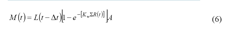
The surface wash-off model is based, as the runoff module, on the single linear reservoir model. The model consists of sediment erosion and its wash-off. First the amount of sediment eroded from the surface and held in suspension in the storm water is calculated. Then the amount of sediment washed into the drainage system is calculated using a single linear reservoir routing method. The amount of sediment washed into the drainage drainage system is calculated as
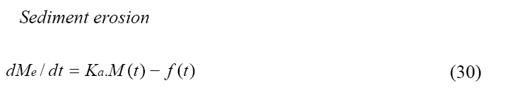
where,
where,
where,
where,
2.4.3. MOUSE Trap
The MOUSE TRAP model provides several submodules for the simulation of sediment transport and water quality for both urban catchments surfaces and sewer systems. Since pollutants are carried by sediment, the model tries its best to correlate sediment transport process and water quality in sewer systems. Mouse Trap can also model the first flush phenomenon based on temporal and spatial distribution of sediment on the catchment surface and sewer system. Surface Runoff Quality (SRQ) computes the pollutant build-up and transport on catchment surfaces. Two major processes that are involved in SRQ are:
1. Build-up and wash-off of sediment particles on the catchment.
2. Surface transport of pollutants attached to the sediment particles.
2.4.4. MUSIC
MUSIC is one of the most popular stormwater model used in Australia developed by Cooperative Research Centre for Catchment Hydrology (CRCCH) Australia (CRCCH 2005).14) The model uses simple first order kinetics for the pollutant wash- off from the surface. According to the model the pollutant concentrations in the parcel tend to move by an exponential decay process towards an equilibrium value for that site at that time.
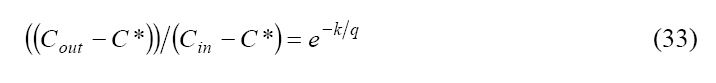
where, Cout is the output concentration, C* is the equilibrium value or background concentration, Cin is the input concentration,
2.4.5. ASTROM
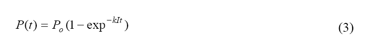
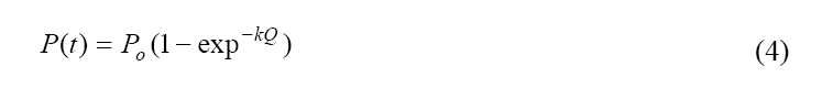
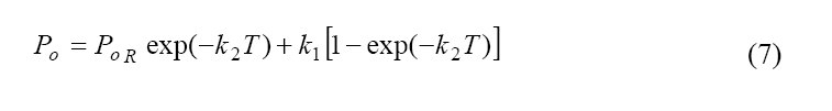
ASTROM model uses the following pollutant build up equation.
where,
Integrating above equation yields
where,
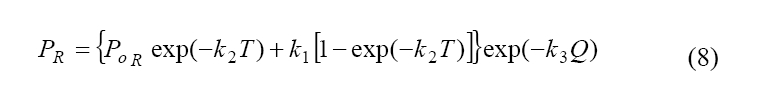
The pollutant washoff model is defined as
where,
The model assumes that rainfall event pollutant wash-off load is proportional to, or dependent upon, the accumulated pollutant mass on the catchment surface before the runoff event, and the pollutant wash-off load is a direct function of runoff volume.
Besides, there are several literatures appeared to describe the wash-off behaviour of pollutants during wet weather period. Here, few are described.
Kim et al., (2005) introduced new wash-off model for highway stormwater runoff that incorporates many parameters such as antecedent dry weather periods, rainfall intensity and runoff coefficient.15) The equation can be initially expressed as
where,
where,
where, δ is an initial concentration related to antecedent dry weather period. The parameters α and γ* are related total runoff. The β* is related to rainfall, runoff coefficient, and storm duration.
This model has two different functions. The first is linear, γ *
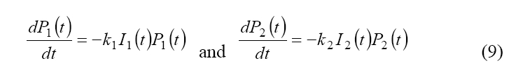
Kanso et al., (2006) applied simple classical pollutant accumulation followed by the wash-off model to describe the water quality.16) He described two accumulation behaviours. The first equation calculates the accumulation of pollutants assumed to follow an asymptotic behaviour that depends on two parameters: an accumulation rate
where,
He described the evolution of the available pollutant mass during the stormwater period by applying the following equation.
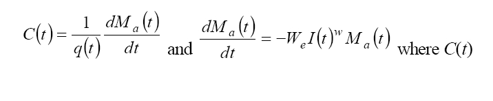
(mg/l) is the SS concentration produced by erosion,
This paper reviews mathematical methods used in stomwater quality modelling and has been undertaken by examining a number of models that are in current use. The analytical techniques are presented in this paper. The important feature of models is discussed.


