The F-region altitudes of the ionosphere are in the range of 150 km to 800 km above ground (http://en.wikipedia. org/wiki/F_region). Vertical profiles of plasma density in the F-region exhibit a maximum altitude of around 350 km (the so-called F-region peak height), and the regions above and below the peak height are commonly referred to as the topside and bottomside, respectively. It has been relatively easy to study the bottomside ionosphere as it can be probed by ionosondes (Park et al. 2013; Kil 2015), which are distributed widely throughout the world. The ionosondes emit radio waves from ground into the ionosphere, and observe reflected waves to estimate vertical profiles of ionospheric plasma density up to the peak height of the F-region. On the contrary, researches on the topside ionosphere are typically more difficult to perform owing to some inherent limitations of ionosondes. One should count on other instruments in order to get information on the topside. Incoherent Scatter Radars (ISRs), for example, can measure the topside plasma moments (Liu et al. 2007). However, there are only a few ISRs in the world, and their duty cycles are generally low because of the high operating costs. Furthermore, ionosondes onboard satellites can sound the topside ionosphere in the same way as the ground-based ionosondes. However, again, only a few topside sounders have been used throughout the history of space exploration (Alouette-1 and Interkosmos-19), and most of which have ceased being in operation long before the year 2000. Radio Occultation (RO) experiments by Low-Earth-Orbit (LEO) satellites, such as CHAllenging Mini-satellite Payload (CHAMP), Gravity Recovery And Climate Experiment (GRACE), and Constellation Observing System for Meteorology, Ionosphere, and Climate (COSMIC), can also give information on the topside plasma density (Liu et al. 2008; Potula et al. 2011). The RO method inverts Total Electron Content (TEC), which is integrated plasma density along the whole line-of-sight between the LEO and the Global Navigation Satellite System (GNSS) satellites, to plasma density at the tangent height. Therefore, the RO method should be applied with caution when horizontal gradient of plasma density is involved(Lei et al. 2007). In summary, it has become a challenging task to investigate vertical profiles of plasma density in the topside ionosphere.

In recent years, a number of studies have attempted to study the topside ionosphere through a combination of multiple observations from ground-based instruments and/or satellites. These studies generally assumed that topside ionospheric profiles can be expressed by one or two analytic functions, and constrain the functions with multiple observations of plasma density and/or TEC. For example, Tulasi Ram et al. (2009) used the alpha-Chapman function constrained by the data from the Republic Of China SATellite-1 (ROCSAT-1) and the ionosondes at a low-latitude and a mid-latitude station. Min et al. (2009) also adopted the same function constrained by data sets from both KOrea Multi-Purpose SATellite-1 (KOMPSAT-1) and Defense Meteorological Satellite Program (DMSP). Stankov et al. (2003) combined the data from ionosondes and TEC into an empirical model for the O+/H+ transition height estimation. These researchers fed the data to several different profilers (i.e., analytic functions) to reconstruct the topside ionospheric profiles.

Though different methods have been used by various researchers to investigate the topside ionospheric profiles, further studies are required in this direction. As mentioned in the preceding paragraphs, the RO technique (Potula et al. 2011) is vulnerable to possible horizontal gradient. ISRs global coverage is poor, and the topside sounders have not been active for decades. These restrictions can be overcome by combining multiple data sets. However, most of the relevant works have investigated only limited regions of the world: near-equatorial regions (Min et al. 2009), one Chinese station at Wuhan (Liu et al. 2014), two stations at Jicamarca and Grahamstown (Tulasi Ram et al. 2009), while others were just dedicated to demonstrating and validating the method (Stankov et al. 2003; Sibanda & McKinnell 2011). In this study, we investigate the topside ionospheric profile around the Korean Peninsula region, which has not been covered thoroughly by the above-mentioned papers. Following the method of Tulasi Ram et al. (2009), we constrain the alpha-Chapman function using data from Korean ionosondes and the Swarm constellation. Section 2 briefly describes the instruments used in this study. Section 3 presents and discusses about the statistical results while Section 4 comes with summary and conclusion.

The Radio Research Agency (RRA) in Korea operates ionosondes in Icheon (37.14° N, 127.54° E) and Jeju (33.43° N, 126.30° E). The F-region peak frequency (foF2) and the F-region peak height (hmF2) at 7-minute cadence are available at the following web site: http://www.spaceweather.go.kr/observation/service/iono. The plasma density at hmF2 (NmF2) can be derived from foF2 by the following equation (http://ccmc.gsfc.nasa.gov/modelweb/ionos/ccir.html):

Note that a similar equation was used in the case study of Yun et al. (2013). European Space Agency (ESA) operates the Swarm constellation that consists of three identical satellites launched on November 22, 2013 into a polar circular orbit. All the three satellites were at the same altitude around 500 km until January 2014, after which orbit maneuver started. In April 2014, the formation flight began and Swarm-Alpha and Swarm-Charlie flew at the same altitude of about 470 km (orbit inclination angle: ~87.3°) with inter-satellite alongtrack separation of about 10 seconds and zonal separation of about 1.5° GLON (Geographic LONgitude). The standalone satellite, Swarm-Bravo, flies about 50 km higher and a slightly different inclination angle (87.7°) compared to two above satellites. The orbit precesses to cover the complete Local Time (LT) sectors in about 131 days. The LT plane of Swarm-Bravo slowly deviates from those of Swarm-Alpha and Swarm-Charlie. Each satellite carries Langmuir Probes (LPs) which can measure electron density, and the data are open to public at the following address: https://earth.esa. int/web/guest/swarm/data-access.

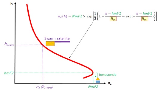
The following is the procedure to estimate the scale height of the topside ionosphere (see also Fig. 1). We note that each ionosonde station (Icheon or Jeju) is treated independently from each other, and each Swarm satellite (Alpha, Bravo, or Charlie) is processed separately as well. Whenever Swarm passes around an ionosonde, adjacent Swarm/LP data points within 5° GLAT (Geographic LATitude) by 5° GLON from the ionosonde station are grouped together, which yields the mean electron density (n_e) per group. For every n_e value, we check whether hmF2 and NmF2 data exist within 8 minutes from the center time of the corresponding Swarm/LP data group on the same date. Then, we use the observed data as the input of the alpha-Chapman function defined as:

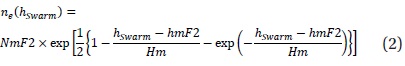
where h_Swarm is the altitude of Swarm, and Hm is the topside scale height. In this equation, the only one unknown parameter is Hm, which can be estimated by the method of substitution. We sequentially input candidate values for Hm (between 0 km and 300 km with step size of 1 km) in order to find the optimal Hm, which minimizes the difference between the Left-Hand Side (LHS) and Right-Hand Side (RHS) of Eq. (2). The Hm is taken as valid only when the minimum difference between LHS and RHS is smaller than 0.005 times NmF2.

We calculate Hm for every day between 09 December 2013 (the first day of Swarm/LP data output) and 30 June 2015. In total 2,256, values of Hm could be retrieved from the Swarm/LP and ionosonde data sets. The statistical distribution of Hm will be given and discussed in the next section.

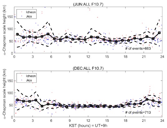
Fig. 2 presents dependence of Hm on the Korean Standard Time (KST). The top, middle, and bottom rows correspond to combined equinox (March, April, September, and October), June solstice (May-August), and December solstice (November-February), respectively. The red and blue symbols show Hm values estimated above Icheon and Jeju, respectively. Black squares represent hourly mean Hm among all the data points from both ionosonde stations (Icheon and Jeju). The black dashed lines stand for one standard deviation above/below the mean. Note that Hm values obtained during periods of geomagnetic disturbance (Kp>3.5) are not shown in Fig. 2.

The dependence of Hm in Fig. 2 on KST and season is, though looking complicated, in qualitative agreement with Fig. 8 of Tulasi Ram et al. (2009), who used the same method of Hm estimation as we do. First, the LT (approximately equal to KST) dependence of Hm is qualitatively consistent. In Fig. 8 of Tulasi Ram et al. (2009) we can identify no salient (i.e., visually identifiable and larger than standard deviations) dependence of mid-latitude (Grahamstown) Hm (denoted by HT in that paper) on LT. Second, Hm in our Fig. 2 (with the mean value mostly around 50 km) is of the same order of magnitude as that of Fig. 8 of Tulasi Ram et al. (2009) although Hm in that paper looks slightly larger (by about a few tens of kilometers) than such values in this study.

Our results do not agree well with results showed in Fig. 2 of Liu et al. (2007), in which Hm values at Arecibo are better aligned with LT than those in our Fig. 2 or in Fig. 8 of Tulasi Ram et al. (2009). The scale height in Liu et al. (2007) generally exhibits (1) post-sunset enhancement for all seasons, and (2) pre-dawn peak except for June solstice (‘summer’ in Fig. 2 of Liu et al. (2007)). The overall level of Hm values in Fig. 2 of Liu et al. (2007) is between 20 km and 80 km, which is of the same order of magnitude as that in this study as well.

We should consider that Hm in Liu et al. (2007) was obtained by fitting electron density profiles from Arecibo ISR between 1966 and 2002. On the other hand, our method (as well as that of Tulasi Ram et al. (2009)) is approximating electron density profiles based only on two observation points (at hmF2 and satellite altitudes). Moreover, our data set only spans about 1.5 years since the Swarm launch. Similarly, Tulasi Ram et al. (2009) investigated mid-latitude Hm during a limited period in 2001-2002. We speculate that the difference of our results (and Tulasi Ram et al. (2009)) from Liu et al. (2007), in terms of the season-LT dependence, can be attributed in part to the approximation method and limited data coverage. However, the day-night difference of Hm in Potula et al. (2011) exhibits significant GLON dependence, which implies that LT dependence of Hm may be different for different GLON. As previous studies investigated Hm by Liu et al. (2007) at Arecibo (GLON: ~66.7° W), Tulasi Ram et al. (2009) at Grahamstown (GLON: ~26.5° E), and ours studied above Korean Peninsula (GLON: ~126.5° E), the GLON difference may also contribute to the inconsistency in Hm among different studies. Further investigations making use of global long-term data sets are necessary in this context.

Differences in Hm between the different ionosonde stations used in this study (Icheon and Jeju) are inconspicuous through an intuitive comparison between the red and blue dots in Fig. 2. This feature may be because the window size of Swarm-ionosonde coincidence (5° GLAT by 5° GLON) is comparable to the distance between the two-ionosonde stations (about 430 km by ~4° GLAT). That is to say, Hm estimated at Icheon (Jeju) may be affected by Swarm/LP data over Jeju (Icheon), which may blur inter-station differences in Hm if any. If we further reduce the window size, the statistical results can become less reliable due to the reduction of data point numbers participating in the Swarm-ionosonde coincidence. Detailed investigation of the inter-station difference can be conducted when more Swarm and Korean ionosonde data are accumulated in the future.

In this study we have investigated alpha-Chapman scale height of plasma density in the topside ionospheric F-region around the Korean Peninsula. The scale height has been calculated from plasma density data of Swarm/LP and foF2/hmF2 data of two Korean ionosondes (Icheon and Jeju) for the period from 09 December 2013 to 30 June 2015. From the statistical distribution of the scale height with respect to LT and season, we can draw the following conclusions:

1. Hm above Korean Peninsula exhibits complex seasonal and LT dependence. The season-LT dependence agrees with that of Tulasi Ram et al. (2009), who used the same method of Hm estimation as ours.

2. The season-LT dependence in this study do not agree well with Liu et al. (2007), who used electron density profiles from Arecibo ISR between 1966 and 2002. The disagreement may be attributed to limitations of our approximation method and data coverage, and inherent dependence of Hm on GLON.

3. The magnitude of Hm above Korean Peninsula is generally around 50 km, which is of the same order of magnitude as those in Tulasi Ram et al. (2009) and Liu et al. (2007).