Operating an Earth-observing satellite at sufficiently lower altitudes can improve its spatial resolution and help a satellite sensor identify smaller details of ground objects. While QuickBird, a typical high-resolution commercial Earth-observing satellite owned by DigitalGlobe, collects the panchromatic imagery at a resolution of 61 cm and an altitude of 450 km, KOrea Multi-Purpose SATellite-2 (KOMPSAT-2) in a 685 km sun-synchronous orbit has a resolution of 1m (Kim 2013). If KOMPSAT-2 were able to observe the ground object at a lower altitude, it could have distinguished more details with a better resolution. However, with the lowering of the operating altitude of a satellite and without a proper altitude maintenance management, the atmospheric drag becomes stronger to ultimately cause its reentry into the Earth. Therefore, for the altitude maintenance of Low-Earth-Orbit (LEO) spacecrafts, fuel-optimal strategy becomes highly critical, as it saves cost and extends the lifetime of the mission as well.
Park et al.(2007) analyzed the effect of drag on orbital variations of KOMPSAT-1 during strong solar and geomagnetic activities. Halbach(2000) presented a numerical study of an optimal periodic thrusting method for LEO spacecrafts using the Legendre-Gauss-Lobatto (LGL) pseudospectral collocation codes developed at Naval Postgraduate School. Park et al.(2008) studied the amount of fuel required to maintain a very low-Earth-orbit with severe air drag using a collocation method. These studies considered air drag as the only perturbation force and acquired solutions using a direct collocation method. However, the actual motion of such satellites in real environments is also affected by other gravitational and non-gravitational perturbations owing to the irregular shape of the Earth (Jo et al. 2011).
In this study, the
The rest of this paper is organized as follows. Section 2 formally presents a fuel-optimal altitude maintenance problem including the objective function, and the governing equations of motion and equality/inequality constraints. Necessary conditions for optimality, such as the costate equations and the transversality conditions are also derived for the indirect optimization method. Section 3 proposes the key process for combining the direct and indirect methods. Section 4 presents simulation results of fuel optimization under various circumstances and the corresponding analyses. Finally, the last section presents the conclusions drawn from the study.
2.1 Altitude Maintenance Problem
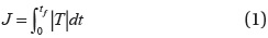
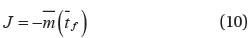
First, an objective function to minimize the fuel consumption is defined as
where
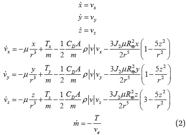
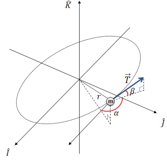
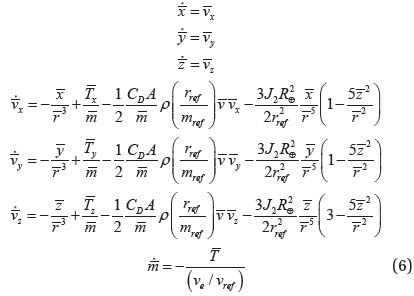
The set of equations under Eq. (2) governs the motion of a spacecraft under the influence of its own thrust, central gravity,
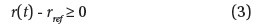
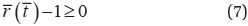
For altitude maintenance, a lower limit is imposed on the altitude as an inequality constraint:

where,

where,

where,

where,
Here
2.2 Necessary Conditions for Optimality
To apply the indirect method, the 1st-order necessary conditions for optimality should be derived. In this case, Eqs. (10) and (11) are used instead of Eqs. (1) and (7), respectively, for simplicity in derivation.
The Hamiltonian is first defined as
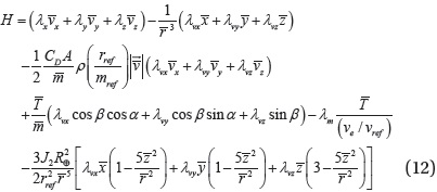
Here, (

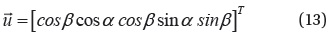
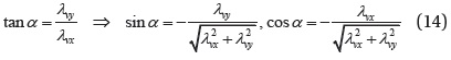
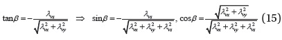
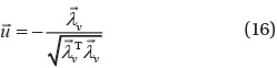
The optimal longitudinal and latitudinal steering can be obtained from the first-order optimality conditions


Note that the (-) sign of the sine and cosine in Eq. (14) comes from the second-order convexity condition

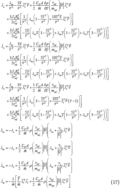
Then, the costate equations are derived from where (∙) represents a general state variable (Kim 2014):

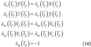
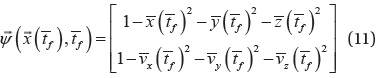
Finally, the transversality conditions are derived as

3. ALTITUDE MAINTENANCE ALGORITHM
In general, a direct method is less sensitive to the initial guess, but shows slow convergence and is not highly accurate. An indirect method converges fast with a proper initial guess of costates, but it is difficult to estimate the initial costates themselves. Given the objective function, governing equation, and associated equality/inequality constraints, the optimal fuel consumption and associated thrust profile are calculated using both pseudospectral (direct) and shooting (indirect) methods. In this manner, a hybrid approach combining the direct and indirect methods is proposed.
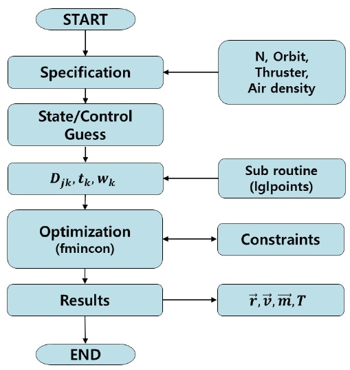
In a pseudospectral method, the state and control variables are approximated at predetermined collocation points (Halbach 2000). In this study, LGL points are used for the discretization of the system, and Lagrange polynomials are used as trial functions (Elnagar et al. 1995). Fig. 2 shows the flowchart of fuel optimization algorithm based on the pseudospectral method (Kim 2014). The input values are the number of LGL points, information of an assigned orbit, physical specifications of a spacecraft and its thruster, and indices associated with air density. In this method, the states and control guesses at the LGL points should be provided. The differentiation matrix (Djk), LGL points (tk), and weights (wk) are determined via a subroutine (lglpoints) (Elnagar et al. 1995). Then, the states and control variables satisfying the constraints while minimizing the objective function are calculated through the ‘fmincon’ in the optimization Toolbox of MATLAB. The ‘fmincon’ attempts to find a constrained minimum of a scalar function of multiple variables starting at an initial estimate (MathWorks 2015a).
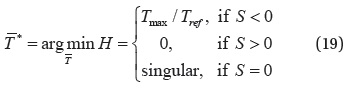
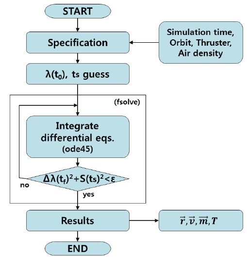
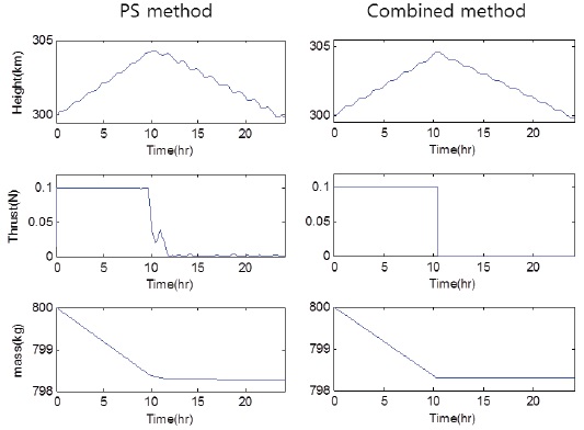
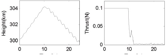
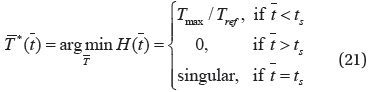
Fig. 3 shows the time history of altitude and thrust profile after applying the pseudospectral method to the fuel-optimal altitude maintenance problem. A spacecraft first ascends with full thrust at the early stage and then descends with null thrust. While the thrust profile is similar to bang-off, it is difficult to precisely determine the switching time by using a pseudospectral method only. This is expected because the optimal switching epoch does not generally coincide with one of the prescribed collocation points of the pseudospectral method. As an attempt to precisely determine the switching time and its associated optimal thrust history, a shooting method is employed with its initial guess obtained from the solution of the pseudospectral method.Fig. 4 shows the flowchart of a fuel optimization algorithm based on a shooting method. Pontryagin’s principle (Pontryagin 1987) yields an optimality strategy for thrust magnitude

Here,

When
The process of updating the initial guesses is iterated until the transversality conditions are satisfied, and this process of solving nonlinear algebraic equations is performed using the MATLAB built-in function, ‘fsolve’. The ‘fsolve’ finds a root (zero) of a system of nonlinear equations (MathWorks 2015b).
4. SIMULATION RESULTS AND DISCUSSIONS
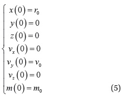
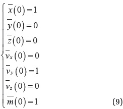
In the altitude maintenance scenario, the assigned altitude is 300 km and a spacecraft starts on the assigned altitude with circular velocity. The physical characteristics of the spacecraft (KOMPSAT-2) and the specifications of the thruster are presented in Table 1.
[Table 1.] Specifications of satellite and its thruster
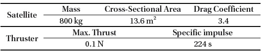
Specifications of satellite and its thruster
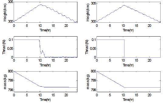
Fig. 5 and Table 2 show that the obscure switching time obtained using the pseudospectral method is precisely determined by applying the shooting method. From the time history of the pseudospectral method, the switching time could be guessed within the range of 9–11 hr. Table 3 shows that a guess selected within this range leads to a proper (local) optimal solution satisfying the altitude maintenance constraints. In contrast, if the guess of switching time is (deliberately) selected outside this range, a non-compatible solution without satisfying the given altitude constraint is generated. This implies that the proposed combined approach can be effectively used for this type of numerically sensitive problems.
[Table 2.] Comparison between results of pseudospectral and combined methods
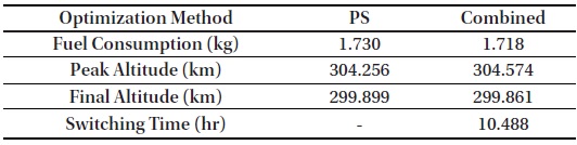
Comparison between results of pseudospectral and combined methods
[Table 3.] Simulation results of pseudospectral method with switching time guess
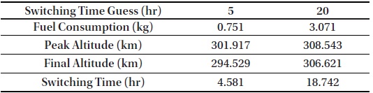
Simulation results of pseudospectral method with switching time guess
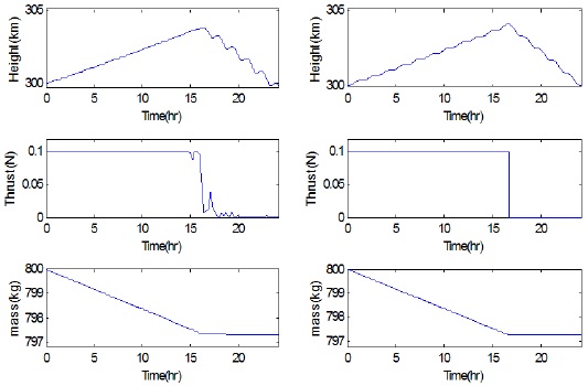
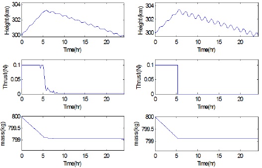
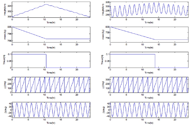
Figs. 6–8 show optimization results with different atmospheric densities (caused by solar activity) using the pseudospectral and combined methods in which the atmospheric model offered by the Australian IPS Radiation & Space Services is implemented (Kennewell 1999). The time for a spacecraft to reach the peak altitude and the switching moment is delayed as the solar activity becomes stronger. For the case of maximum solar activity (Fig. 6), the spacecraft raises its altitude for about 2/3 of the operation time, and then drops rapidly for about 1/3 of the operation time owing to the high atmospheric density. In contrast, when solar activity is weak (Fig. 8), a spacecraft reaches the peak altitude at about 1/4 of the operation time, and then descends slowly for the remaining operation time. Fuel consumption for the case of maximum solar activity is about three times larger than that for minimum solar activity (Table 4).
[Table 4.] Comparison between results of pseudospectral and combined methods for solar activity
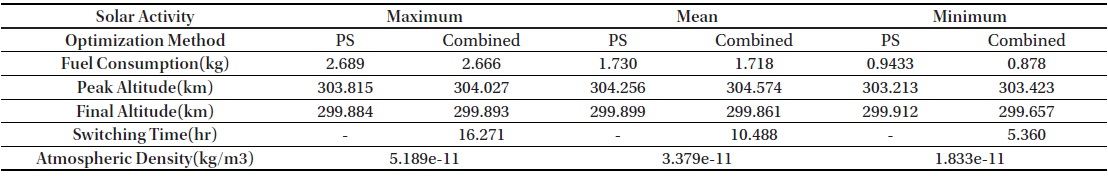
Comparison between results of pseudospectral and combined methods for solar activity
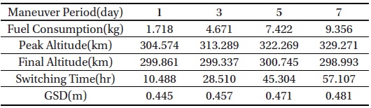
Table 5 shows optimization results with different maneuver periods. Fuel consumption increases with the maneuver period, but this increase is not proportional. For example, the fuel consumption for 5 days is less than that for 1 day multiplied by 5. This is because a spacecraft reaches higher altitude where atmospheric density is lower when the maneuver period is longer. KOMPSAT-2 collects panchromatic imagery at 1m resolution with Instantaneous Field of View (IFOV) 1.46 μm at an altitude of 685 km. Based on the IFOV of KOMPSAT-2, Ground Sampling Distance (GSD) is calculated using the relation between GSD and altitude (Park et al. 2008). GSD could be improved to be under 0.5 by lowering the altitude of spacecraft.
[Table 5.] Simulation results of combined method with maneuver period

Simulation results of combined method with maneuver period
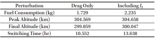
Fig. 9 shows simulation results considering the
[Table 6.] Simulation results of combined method with J2 perturbation

Simulation results of combined method with J2 perturbation
Pseudospectral and shooting methods were combined to optimize the fuel consumption for altitude maintenance of spacecrafts at 300 km circular orbits where atmospheric drag is sufficiently strong to cause orbital decay. Based on the physical characteristics of KOMPSAT-2, simulations showed that a satellite ascended with full thrust at the early stage and then descended with null thrust. While the thrust profile was similar to bang-off, it was difficult to precisely determine the switching time by using only a pseudospectral method. As an attempt to precisely determine the switching time and its associated optimal thrust history, a shooting method was employed with its initial guess obtained from a solution using the pseudospectral method. By analyzing the results with solar activity, fuel consumption during the maximum solar activity was found to be three times more than that during the minimum solar activity. This implies that the solar activity cycle is a critical factor while designing a LEO mission. Furthermore, fuel consumption was reduced when the maneuver period of satellites was increased. This is possible because with extended maneuver periods, satellites reach higher altitudes where the atmospheric drag is relatively weak. For the case considering
The overall hybrid process proposed in this paper can provide a robust, efficient, and precise fuel-optimal solution for various cases of satellite maneuvers.