An important problem in extreme ultraviolet lithography (EUVL) is the detection and characterization of defects on multilayer masks [1]. The fine structures of a mask present features much smaller than the wavelength, hence conventional imaging methods cannot provide images with sufficient resolution.
One proposed approach relies on coherent diffraction [2, 3]. A coherent beam is projected onto the mask, and the diffraction pattern is measured. As a result, the information obtained is not directly the shape of the mask but instead the modulus of its Fourier transform. Phase information is lost, but it is possible to recover it by a phase retrieval method if the sampling frequency is high enough. The principle of the phase retrieval algorithm is to go back and forth between real and frequency domains and apply constraints such as positivity, finite support, or the given Fourier transform magnitude in these two respective spaces. Several phase retrieval algorithms with different types of constraints have been proposed [4]. The most widely used is the hybrid input-output (HIO) algorithm, as it enables converging to a global minimum. Unfortunately, in the presence of noise, convergence may be very slow, and in practice, solutions tend to oscillate as a function of the number of iterations because separate constraints in the real- and Fourier- spaces cannot be satisfied at the same time. Several solutions have been demonstrated to make the phase retrieval algorithm more robust to noise, such as the oversampling smoothness method [5], but they still suffer from some limitations. Kim
Another suggested approach is the deterministic method. In this case, control data are needed, such as from a defectfree mask. For example, Taylor proposed an off-axis holography technique by adding a point signal far off the region of the support of the desired signal [8]. Fienup has considered the reconstruction of signals having latent reference points [9]. Fiddy
In this paper, we consider the application of a deterministic algorithm for this problem. First, we assume that the mask has an L/S pattern and that the diffraction pattern of the original defect-free mask is available. Secondly, we assume that the shape of the defect is a single stripe and is located on the left of the mask. This assumption is not critical because the diffraction pattern is preserved against some transforms including translation, especially reflection, in particular time-reversal for a one-dimensional signal. The goal is to estimate the location and shape of a stripe defect and distinguish it from the diffraction pattern of a defect-free mask. Contrary to iterative approaches, our method enables the determination of the exact shape of a defect, including its position and depth. The reconstruction of the defect-free mask may be important in the sense that we need to check whether the structure of the real mask, which is referred to as a reconstructed defect-mask in this paper, has the same structure as the one that we had designed and known structure. Also, although in many cases we have some knowledge on the shape of the defect-free mask, when we use a mask pattern for the first time, we need to determine the exact shape of it to compare whether the real one has exactly the same structure that we had designed and intended to have.
This paper is organized as follows. In Section II, we describe the problem and a mathematical model as a solution. In Section III, we derive equations for determining the values of interest. In Section IV, we show an example demonstrating the validity of the algorithm.
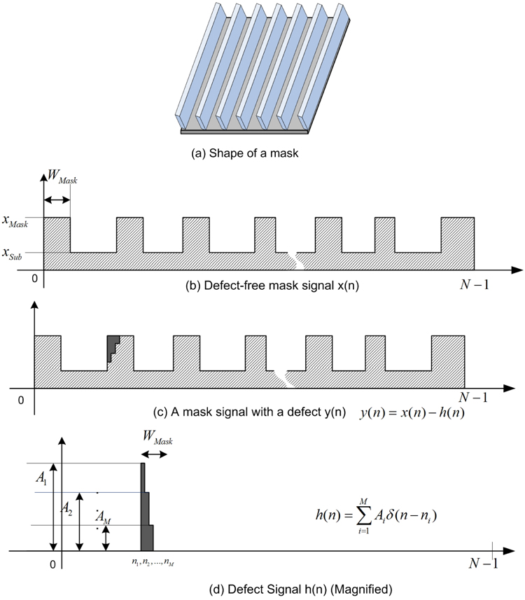
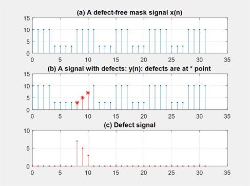
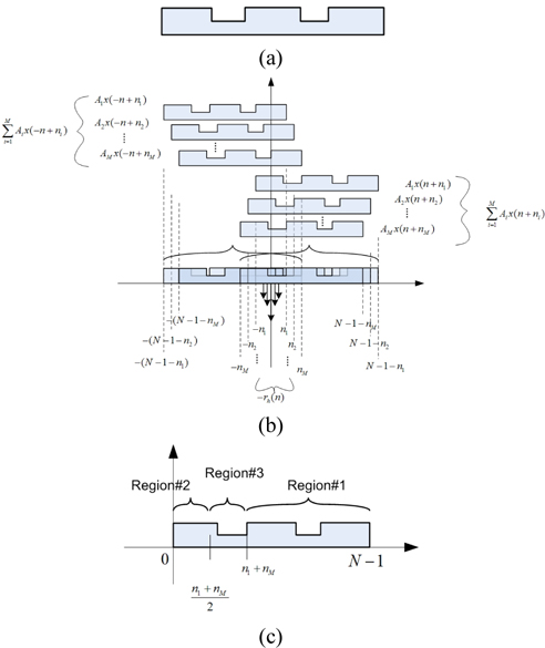
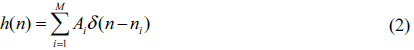
We consider a simple stripe-type defect that occurred in an L/S-type pattern mask [1]. Figure 1 is a shape and model of such a mask and a defect. Figure 1(a) is the shape of a defect-free mask and (b) is the cross-section of this mask on the x-y plane. We let the mathematical notation of the defect-free mask model be

where
where
For convenience, we assume that all
In this section, we derive equations for the calculation of the values of
3.1. Mathematical Preliminaries
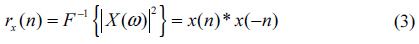
3.1. Mathematical Preliminaries We assume that we have a prior knowledge of the diffraction pattern of the defect-free mask pattern. Then, if we take the inverse Fourier transform of the diffraction pattern, we can get the autocorrelation function of the mask pattern signal. In mathematical terms,
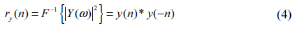
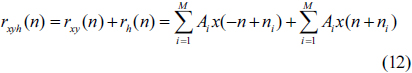
Likewise, if we get the inverse Fourier transform of the square of the diffraction pattern of the defected signal

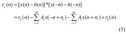
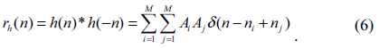
Using relationship (1), the autocorrelation function

where

Here,
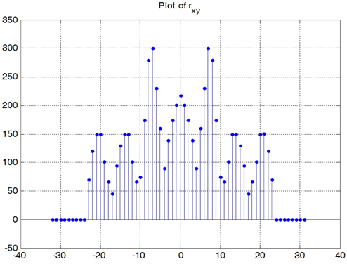
If we plot this
3.2. Determination of Boundary Values xmask
The boundary value
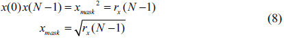
From this equation, we determined two boundary values
Since we do not know the exact shape of the defect-free mask signal, we need to devise some ways to determine the location of the defects. From Fig. 2(b), which shows the structure of
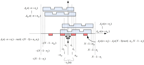
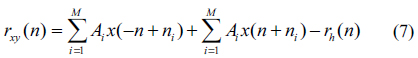
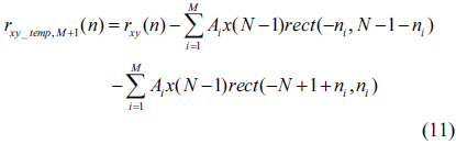
The remaining values can be determined as follows. If we subtract
then we can erase the effect of the first term

where and
has no values greater than 0.
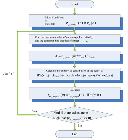
Consequently, we are able to determine the location and amplitude of all defects. We can represent the defect profile the same as the equation given in Eq. (2). Figure 4 is the block diagram of the algorithm for estimating the defect signal.
3.4. Reconstruction of the Mask Structure
Since in 3.3, we have determined the defect signal, now we can reconstruct the defect-free mask signal
In Fig. 2(c), we have divided the support of the mask pattern into 3 regions. The reconstruction may be done in 3 steps.
3.4.1. Region #1
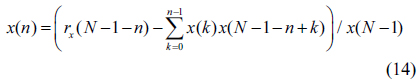
The range of Region #1 covers the indices of [
Using this equation recursively, we determine the values of x(n) as

for
3.4.2. Region #2
The range of Region #2 covers the indices of
for
3.4.3. Region #3
The values of the mask pattern in Region #3 starting from +1. to (
for
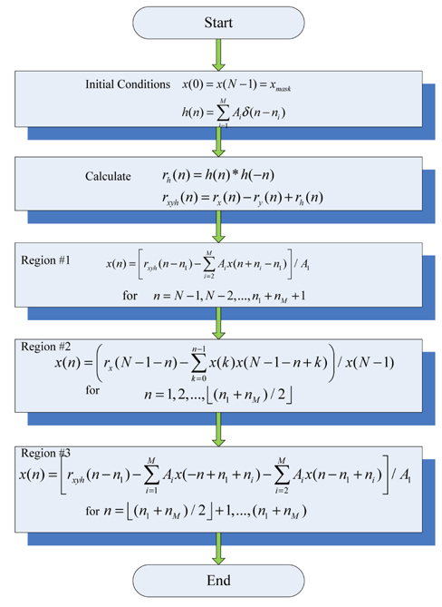
Summarizing these 3 equations, we can reconstruct the entire values of the mask pattern. In Fig. 5, we have summarized these equations into an algorithmic block diagram. In the next section, we present an example that shows the validity of this algorithm.
In this section, we demonstrate the validity of the equations with an example.
We assume that
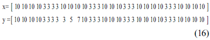
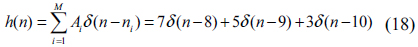
From this, the defect is given as a signal

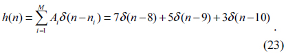
which, using the delta notation as in Eq. (2), can be represented as

Here,
Using these values, we calculate the values of the diffraction patterns of the two mask patterns
[TABLE 1.] Values of the autocorrelation functions and its difference
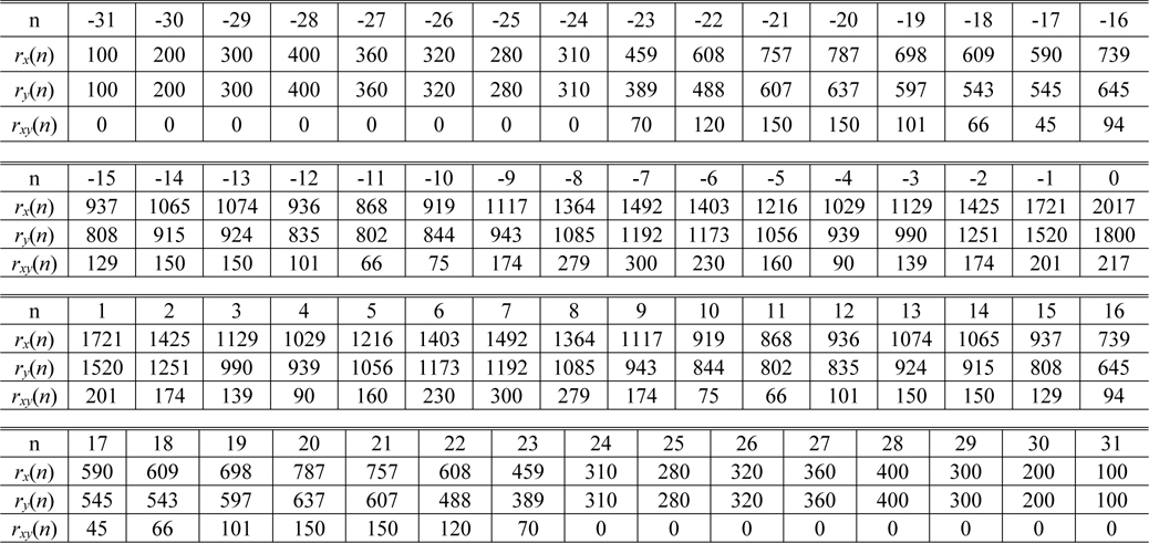
Values of the autocorrelation functions and its difference
4.2. Determination of the Boundary Values
From Table 1 and Eq. (8), we determine the boundary values from

4.3. Determination of the Defect Signal h(n)
As can be seen in Table 1 as well as in Fig. 7, the support of

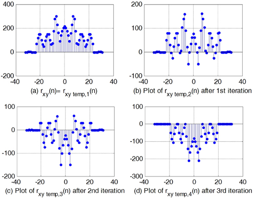
To determine the size and location of the next defect points, we need to calculate
As we can see in Fig. 8(b), the boundary value is at

Similarly we get

If we calculate
From this, we can calculate its autocorrelation
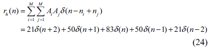
With this, we can calculate
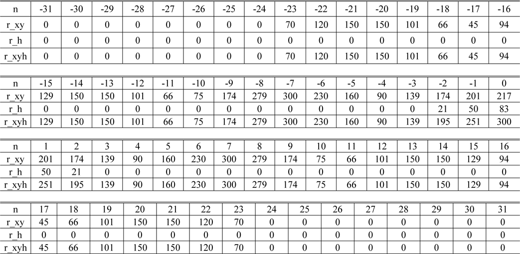
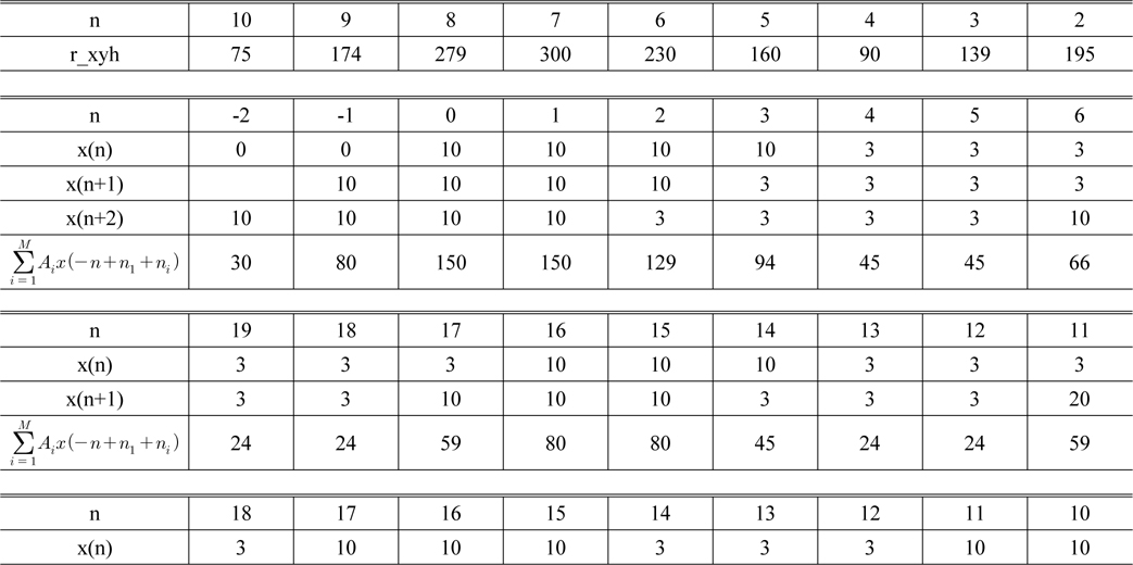
[TABLE 2.] Values of the signals rxy(n), rh(n), rxyh(n)

Values of the signals rxy(n), rh(n), rxyh(n)
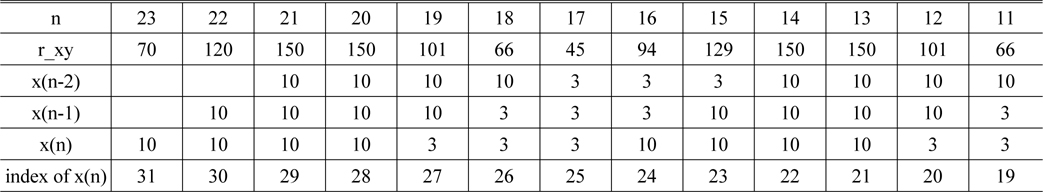
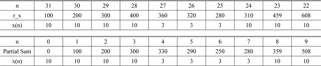
[TABLE 3.] Values of the mask pattern in Region #1

Values of the mask pattern in Region #1
[TABLE 4.] Values of the mask pattern in Region #2

Values of the mask pattern in Region #2
4.4. Reconstruction of the Defect-free Mask Signal x(n)
The mask signal can be reconstructed as follows:
4.4.1. Region #1
In Region #1, the signal can be reconstructed using Eq. (13).
4.4.2. Region #2
The values of mask pattern in Region #2 can be obtained from the definition of the autocorrelation function of the mask signal
4.4.3. Region #3
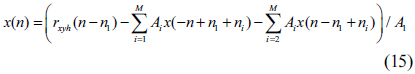
The values of the mask pattern in this region can be obtained by using Eq. (15).
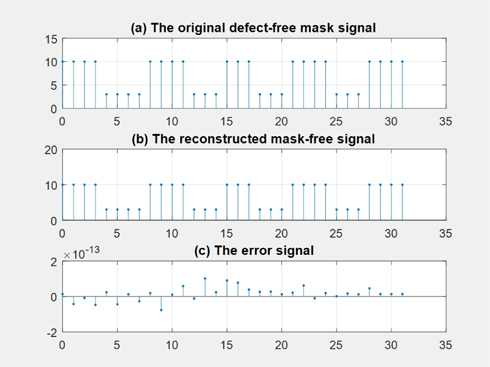
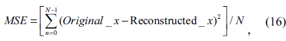
Collecting all these values, we can reconstruct the defect-free mask pattern and is shown in Fig. 9. In this figure, we also compared the original defect-free mask signal and the reconstructed signal. The last figure shows the error signal between the original signal and the reconstructed signal. If we define the mean square error as

then the MSE is given 1.6916×10⁻²⁷ in this case and the difference between the original signal and the reconstructed signal is less than 1×10-13, which is not significant considering calculation errors.
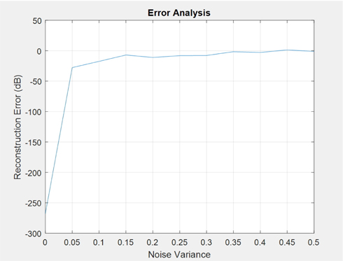
In Fig. 10, we have presented an error analysis with respect to the measurement noises. The x-axis and y-axis show the variances of noises that are added to the measured diffraction pattern values and the mean squared error in dB calculated using Eq. (16), respectively. As we can see in this figure, if noises are inserted, it influences the performance of the algorithm. This is true for the many closed-form phase retrieval algorithms [15]. However, in this case we can see that the effect of the measurement error is not much dependent on the noise level if the noise-level is below a certain level.
[TABLE 5.] Values of the mask pattern in Region #3
Values of the mask pattern in Region #3
In this paper, we considered a method for the estimation of the location and the amount of stripe-type defect in an L/S type mask and the reconstruction of a defect-free mask in lithography. First, we derived an algorithm to estimate the location and depth of the defect signal. Secondly, we derived a deterministic algorithm for the reconstruction of the defect-free mask signal. Using the estimated defect signal and defect-free mask signal, we could also estimate the mask signal with the defect. We present an example that proves that the algorithm works.
It is known that the EUVL is important in developing nanoscale semiconductor chips. The main contribution of this paper is that if we have a defect-free as well as a slightly defected mask pattern, then by measuring the diffraction patterns of these two mask patterns, not only we can estimate the shape and the location of the defect but also determine the exact shape of the defect-free mask pattern. Also, we can use this method for comparing two mask patterns; not only we can find the difference but also we can reconstruct the exact shapes of the two mask patterns, which may be used in the automatic detection /classification of defected masks.