Magnetic bearings use magnetic force to levitate a rotating shaft without contact friction. Compared to conventional fluid-film and rolling element bearings, magnetic bearings have the advantages of no lubricant, high rotation speed and long-life. Magnetic field is the physical medium to realize magnetic bearings’ levitation and motion control, and the air-gap flux density distribution essentially determines the coil/geometry-forces relationship and influences magnetic bearings’ operation performance.
Due to the essential open-loop instability of magnetic bearings [1], the control currents are being adjusted to pull the rotor to the desired position continually, which results in varying magnetic field. The varying magnetic field results in eddy current and hysteresis effects, which cause considerable magnitude reduction and phase lag of bearing stiffness. Therefore, characterization of the dynamic magnetic field of magnetic bearings is important for enhancement of bearings’ operation performance.
Normally, characterization of the dynamic magnetic field of magnetic bearings merely relied on theoretical analysis with analytical methods or finite element methods. For example, Bostjan Polajzer
However, there are few researchers who performed the measurement of dynamic magnetic field in magnetic bearings to validate the theoretical analysis and simulation. The main possible reason is that it is difficult to mount the conventional Hall-effect magnetic field sensors in the air-gap, which is normally no more than 2 to 3 mm thick. Moreover, it is infeasible for Hall sensors, a type of separate sensor, to construct a sensor array to get the spatial distribution of the rotating field in the constricted space of a magnetic bearing’s air-gap.
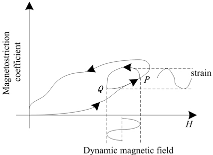
To solve the above problems, a fiber Bragg grating-Giant Magnetostrictive Material (FBG-GMM) magnetic sensor was proposed in this paper. As the FBG only responds to the mechanical and thermal loading, it cannot detect the magnetic field directly. Giant Magnetostrictive Material (GMM), which is a magnetic-machinery conversion material, is usually used with an FBG to form a magnetic field sensor. GMM is a new functional material which experiences length deformation along its magnetization direction in the external magnetic field, when the external magnetic field returns to zero, its length is restored to the original value and this phenomenon is called the magnetostrictive effect. In all the Giant Magnetostrictive Materials, the synthetic material which consists of terbium(Te), dysprosium(Dy) and iron(Fe) in specific proportion is the most widely used due to its reliable performance, large magnetostrictive coefficient (which is over 1000 along its major axis) and it is also widely used in the field of actuators, current sensing, sonar systems and so on.
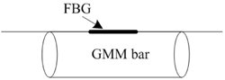
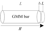
The typical configuration of FBG-GMM magnetic field sensor is shown as Fig. 1. A FBG is attached onto a GMM rod along its principal magnetostriction orientation to detect the GMM rod strains when it is exposed to a magnetic field.
Recently many researchers investigated the properties and applications of FBG-GMM magnetic sensors in magnetic sensing. In reference [7], the FBG-GMM sensor was used in an electric transmission line to study the magnetic field interference. In reference [8], an FBG-GMM sensor was used to measure the large power current, and the linear relationship between the current and the wavelength was calibrated. In reference [9], a low-cost fiber Bragg grating optical current transducer based on magnetostrictive material was presented, the experiments demonstrated that the sensor could be used in the currents in the range of 320-900 A while the temperature ranged from 25℃ to 45℃. In reference [10], an FBG-GMM sensor was used to measure AC current from 0.3 A to 1 A in the temperature range from 18℃ to 90℃. In reference [11], an FBG-GMM sensor was used to measure the dynamic current of 50 Hz and research was also done on improving the linearity of the FBG-GMM sensor. In reference [12], a 10 mm FBG-GMM sensor was presented under the condition of current from 0 to 3 A, and the results showed its linear property was improved after loading certain biased magnetic fields. In reference [13], a magnetic field sensor was proposed to measure the static and dynamic magnetic field in the air-gap of electric generators while the FBG was coated by a layer of magnetostrictive composite. In reference [14], the FBG-GMM sensors were proposed to measure current ranging from -170 A to 170 A. In reference [15], GMM and the MONEL400 metal alloy were bonded on the same FBG to be a current sensor. The sensor was used to measure both DC and AC currents. In reference [16], a linear magnetic actuator of which the core material was GMM and a cantilever beam were used with FBG to be a current sensor, the result showed the sensor had good linearity and repeatability.
In the recent research on FBG-GMM sensors, the FBG was always attached along the principal magnetostrictive direction to the GMM rod or bar, and to get enough bonding, the GMM rod or bar should be longer than the FBG whose length is normally about 8 mm to 10 mm. So the FBG-GMM sensors commonly have the length varying from 15 mm to 30 mm. This scale is capable of being used in electric current sensing; however, it is impossible to use it for magnetic field sensing in small gaps, which may be prevalent situations in a magnetic bearing’s magnetic field measurement.
In this paper, a novel thin GMM-FBG magnetic field sensor for magnetic bearings was designed and studied. A calibration experiment for the sensor was proposed. A magnetic field sensor was used in the air-gap of magnetic bearings to measure the dynamic magnetic field. During the dynamic experiment, magnetic fields with different frequencies from 30 Hz to 300 Hz with the interval of 30 Hz were applied on one pole of the magnetic bearings. Through comparing with the finite element simulation simulations, the results showed the DC component of the dynamic magnetic field in the magnetic bearings’ air-gap can be measured by the FBG-GMM sensor.
2.1. Principle of Fiber Bragg Grating Sensing
The sensing principle of FBG is based on demodulating the wavelength of the reflective light signal in the optical fiber. When broadband light transmits to the FBG through the optical fiber, a narrow-band component is reflected back.
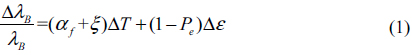
The reflected Bragg wavelength is sensitive to the temperature and the strain. It can be expressed using Eq. (1):

Where
In general,
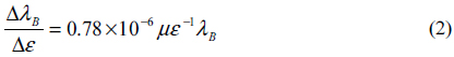
From Eq. (2), it can be concluded that for every 1
For silica fibers, the thermal response of FBG is dominated by the variable ξ. When the strain effect on FBG is constant, the relationship between Δ
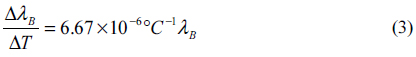
From Eq. (3), it is found that for each 1℃ increased effect on FBG, the reflected Bragg wavelength increases 8.67
2.2. Magnetostrictive Effects of GMM
Some magnetostrictive materials, such as
2.3. The FBG-GMM Magnetic Sensor
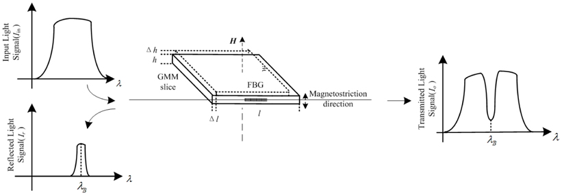
Different from the typical FBG-GMM sensor in which FBG was usually bonded along the major magnetostriction direction of GMM, in this paper FBG was bonded perpendicular to the major magnetostriction direction of GMM. When the sensor was placed in the small air-gap, as the direction of the magnetic field is shown in Fig. 3, the sensor experienced deformation along its thickness direction(
For the GMM slice, first
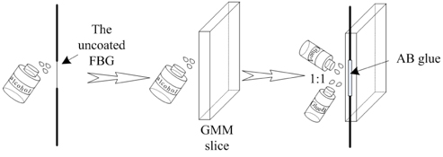
This section mainly describes the attaching procedures for the FBG-GMM sensor. For the GMM slice, alcohol was used to clean the large flat side. For the FBG sensor, the coating layer was removed and alcohol was also used to clean the uncoated FBG. The AB glue, which was mixed with the proportion of one-to-one, was used to attach the FBG on the cleaned side of the GMM, then allowed to stand for one day until the glue cured. Finally, the FBG-GMM sensor was finished as shown in Fig. 4.
3.2. FBG-GMM Sensor’s Static Calibration
Since the magnetostriction of the
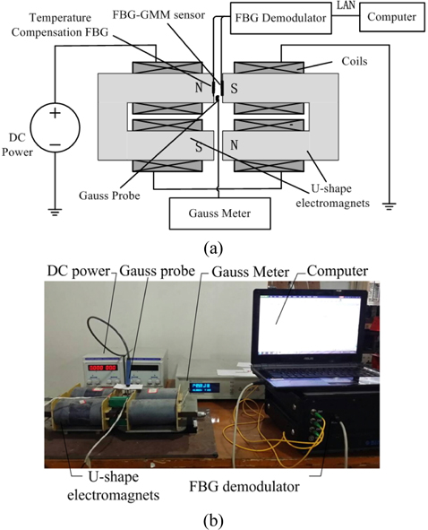
Figure 5 shows the FBG-GMM sensor’s calibration experiment system. The calibration experiment system was composed of a pair of U-shape electromagnets, a DC power supply, a FBG-GMM magnetic sensor, a temperature-compensation FBG sensor, a Gauss meter and a FBG wavelength demodulator connected with the computer. The two U-shape electromagnets were series connected and each U-shape electromagnet was made of 30 stacked pieces of 0.5 mm-thick silicon steel lamination wrapped with 800-turn coils. The air gap between the two electromagnets was fixed at 4 mm. The FBG-GMM sensor (the central wavelength was 1286 nm) was bonded onto the surface of one magnetic pole to measure the flux density in the air gap while the temperature-compensation FBG sensor (the central wavelength was 1316 nm) was bonded on the opposite pole to monitor the temperature variation. These two sensors were respectively connected to the different channels of the same FBG wavelength demodulator, which is fast enough to catch the AC magnetic field due to its 4000 Hz sampling frequency. The probe of the Gauss meter was placed in the air gap to measure the magnetic flux density to calibrate the FBG-GMM magnetic sensor. The DC power supply applied DC current on the electromagnets to form a static magnetic field in the air gap. During the calibration experiment, DC current varied from 0 to 2.5 A with an interval of 0.1 A.
The wavelength shift of the FBG-GMM sensor resulted from two parts: the strain caused by magnetostriction and the temperature variation. The wavelength shift caused by the magnetostriction can be calculated by Eq. (4):
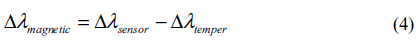
In Eq. (4), Δ
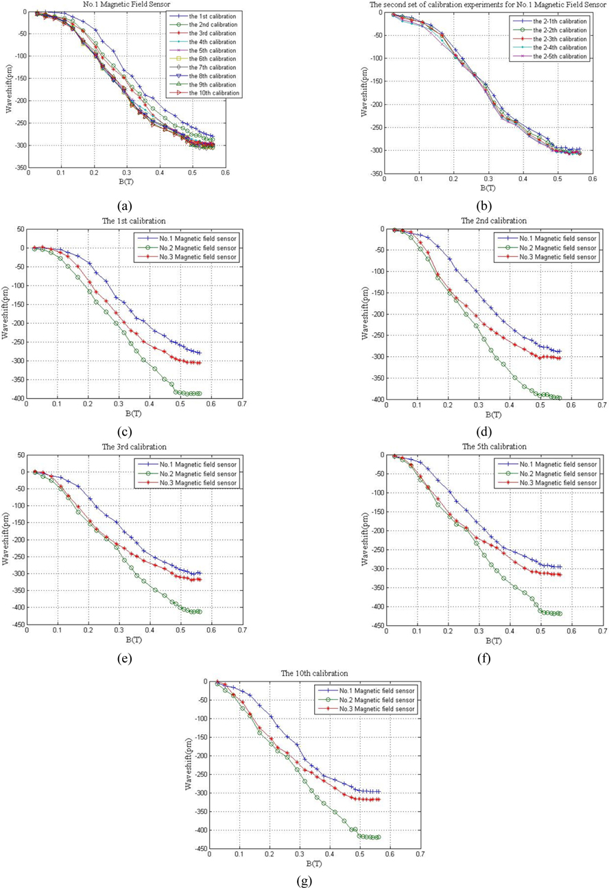
Three FBG-GMM sensors were calibrated and each sensor was calibrated 10 times, the calibration results are shown in Fig. 6.
From Fig. 6(a), it can be seen that the calibration curves converged to the 10th calibration curve, due to the residual magnetism effect of GMM. At the next day of 10 times calibrations, 5 more calibrations which show in Fig. 6(b) were done to get more accurate performance of the No.1 magnetic field sensor. By comparing Fig. 6(a) with Fig. 6(b), the average calibration curve of the 3rd~10th calibration curves in Fig. 6(a) are more accurate to describe the No.1 magnetic field sensor’s performance. By comparing Fig. 6(c) ~ 6(g), the sensor performance is different for each calibration, this is because the sensor performance differs as not only the Possion’s ratio [18] of GMM but also the thickness, width, length of the adhesive [19] which all relate to strain transfer between GMM and FBG.
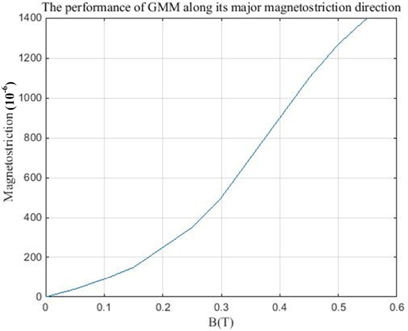
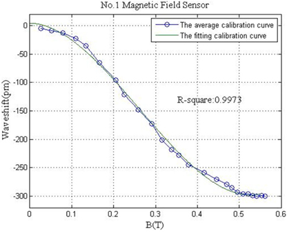
Figure 7 shows the performance of GMM [20] along its major magnetostriction direction, with external magnetic field increasing, the major magnetostriction direction of GMM elongates while its length-direction gets compressed which meets the performance of the magnetic field sensor. The average calibration curve is calculated by the 3rd~10th calibration curves in Fig. 6(a) and it can be divided into two parts, the first part was from 0
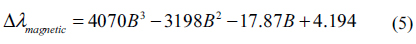
The fitting calibration curve of No.1 magnetic field sensor which was used in the following experiments can be described by Eq. (5):

3.3. Simulation and Measurement
In this section, simulation of the magnetic flux density distribution in the air-gap of the magnetic bearing with dynamic current was implemented and the air-gap dynamic flux density measurement through the FBG-GMM sensor was performed.
The magnetic bearing was of an 8-poles NNSS coil configuration and the air-gap was fixed at 2.5 mm. The magnetic bearing had a symmetrical structure, which resulted in symmetrical magnetic field distribution, and each pole pair had the same flux density. Based on this premise, a pole pair containing pole 6th and 7th was chosen to perform the dynamic magnetic field simulation and measurement. Coils of pole 6th and 7th were loaded on the dynamic current while the rotor remained stationary. The dynamic current applied on coils can be described by Eq. (6).

In Eq. (6),
Assuming the system was linear, based on the dynamic current of the coils, the dynamic magnetic flux density can be described by Eq. (7).

Where
3.3.1. FEM Simulation
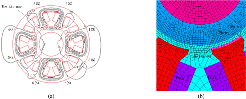
In the simulation, the finite element method analysis based on ANSYS was proposed. In Fig. 9(a), it shows the distribution of the magnetic flux line and it could be found that the magnetic field distribution of 8 poles in the air-gap was symmetric. The simulation model was meshed as Fig. 9(b). There were 21 simulation points on the pole 7th which were set to simulate the magnetic flux density in the air gap. Based on the installing location of the FBG-GMM sensor, point 8 in the simulation corresponded to the FBG-GMM sensor in the dynamic experiment.
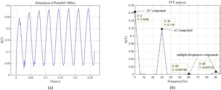
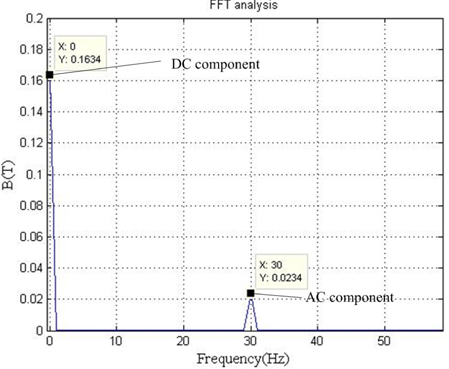
Figure 10 shows the simulated magnetic flux density at the location of the FBG-GMM sensor (Point 8). Figure 10(a) shows the time-variant curve of the magnetic flux density with the dynamic current of 30 Hz. In Figure 10(b), DC component and AC component of the flux density were retrieved by FFT analysis. From the FFT analysis, the multiple-frequencies components in the flux density have much smaller amplitude than its main frequency (AC component), there was an assumption that the system was linear and only the DC and AC components were used to analyze the performance of the sensor.
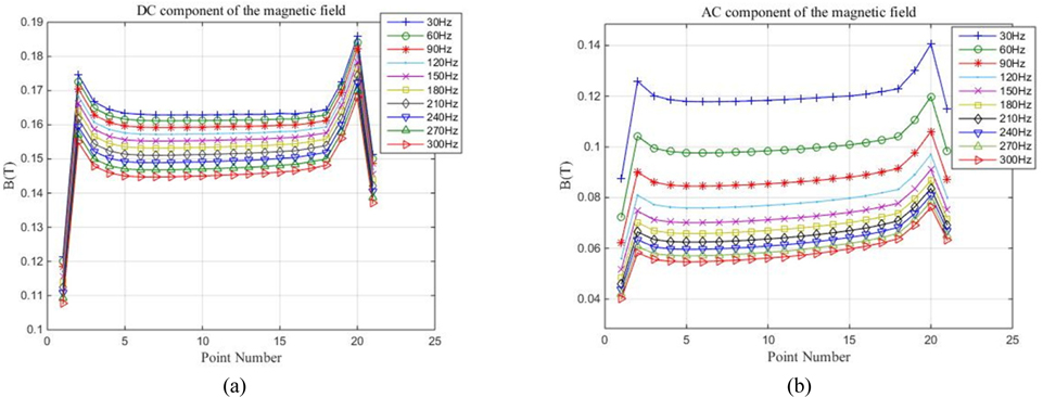
Figure 11 shows the circumferential distribution of the air-gap flux density from 30 Hz to 300 Hz of the pole 7th based on the simulated results of the 21 points in the mesh model. Figure 11(a) and Figure 11(b) show the DC component and AC component of the air-gap flux density respectively.
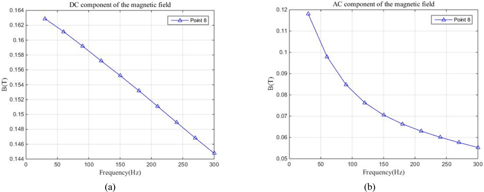
With the frequency of the magnetic field increased from 30 Hz to 300 Hz, the DC component of the magnetic flux density of Point 8 linearly decreased by 0.0181 T from 0.1629 T to 0.1448 T in Fig. 12(a), while the AC component of the magnetic field decreased by 0.0627 T from 0.118 T to 0.0553 T in Fig. 12(b).
3.3.2. Measurement
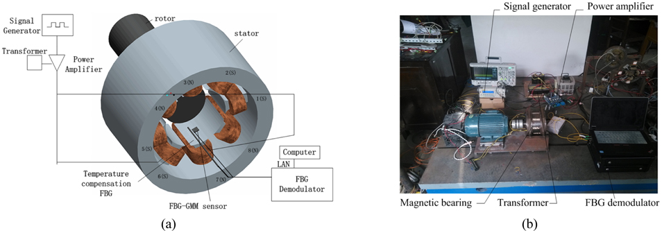
In the measurement, the setting of the current applied on coils was in correspondence with the simulation. The dynamic experiment system was composed of a signal generator, a transformer connected with the power amplifier to get wide working frequency of the power amplifier, a power amplifier used to generate the dynamic current applied on the coils, temperature-compensation FBG, the FBG-GMM sensor and the FBG demodulator connected with the computer. The schematic diagram and system of the dynamic magnetic field experiment is shown in Fig. 13.
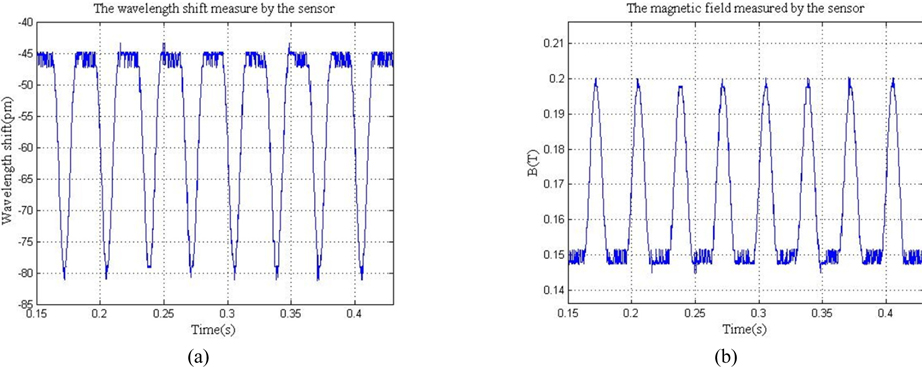
Figure 14(a) shows time-domain signal of the measured wavelength shift while Fig. 14(b) shows the time-domain signal of the measured magnetic field, and the FFT analysis of the magnetic field measured by the sensor is shown in Fig. 15.
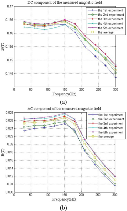
The experiments were repeated five times, and the average DC component and the average AC component of the magnetic flux density are shown in Fig. 16. With the frequency of the magnetic field increased from 30 Hz to 300 Hz, the average DC component of the measured magnetic field decreased by 0.0172 T from 0.1635 T to 0.1463 T while the average AC component of measured magnetic field decreased by 0.0142 T from 0.0253 T to 0.0111 T.
In this section, the results of the simulation and measurement are discussed from the perspective of DC component and AC component.
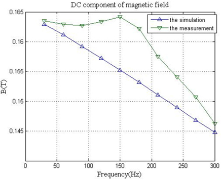
From Fig. 17, as the frequency increased from 30 Hz to 300 Hz, the magnetic flux density in the simulation decreased by 0.0181 T from 0.1629 T to 0.1448 T while the magnetic field in the measurement decreased by 0.0172 T from 0.1635 T to 0.1463 T on the DC component. In the measurement, when the frequency increased from 30 Hz to 150 Hz, the measured magnetic flux density changed slightly and when the frequency increased from 150 Hz to 300 Hz, the measured magnetic flux density changed significantly, which causes the output strain of GMM to linearly decrease with the external magnetic field. The reason is that the
In Table 1, it shows the error of the measurement is less than 5.87%, which is accurate for measuring the magnetic field in the air gap of magnetic bearings from the perspective of DC component.
[TABLE 1.] DC component error analysis
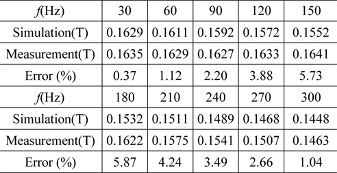
DC component error analysis
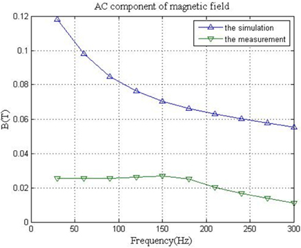
Considering from AC component, the magnetic flux density in the simulation decreases by 0.0627 T from 0.118 T to 0.0553 T while the magnetic field in the measurement decreases by 0.0142 T from 0.0253 T to 0.0111 T in Fig. 18. It shows that the measured AC component of the magnetic flux density differs greatly from the simulation. The primary reason is that
An FBG-GMM magnetic field sensor for magnetic bearings was presented and applied to measure the magnetic flux density in the air-gap between the rotor and stator. In the sensor, the FBG was attached perpendicular to the principal magnetostriction orientation of a GMM slice, which solved the problem that the commonly used FBG-GMM sensors cannot be used for magnetic field measurement in small gaps. The result of the calibration experiment indicated that the performance of thin-slice FBG-GMM sensor can be described by a polynomial curve. Experiments on magnetic bearings were implemented to test the property of the FBG-GMM magnetic field sensor and the measurement was compared with the finite element simulation. The results showed the error was less than 5.87%. The sensor was feasible for measuring the DC component of the dynamic magnetic field in magnetic bearings. But the AC component of the dynamic magnetic field was hard to detect accurately. The next steps focus on minimizing the effect of hysteresis effect on dynamic magnetic field measurements to accurately measure the AC component of the dynamic magnetic field in magnetic bearings.