Photoelasticity is an experimental method for analyzing stress or strain fields in mechanics [1]. Non-crystalline transparent materials, such as polymeric plastics, are optically isotropic under normal conditions but become doubly refractive when stressed. This basic physical characteristic of photoelasticity was first observed by Brewster in 1816 [2]. The method of photoelasticity allows one to obtain the principal stress difference and the principal stress direction in a model. The principal stress difference and the principal direction are presented as isochromatic and isoclinic, respectively [3]. In 1990, Brown and Sullivan [4] introduced use of polarization stepping for whole field isoclinic determination in a plane polariscope with a monochromatic light source. Petrucci [5] utilized the optical arrangement of Brown and Sullivan and replaced the monochromatic light source with a white light source. Lei et al. [6] concluded that the isoclinic parameters obtained using white light gave better results. Plane polariscope based algorithms are better for isoclinic parameter evaluation [7, 8]. A polarization stepping method in white light has been effectively used to determine that the isoclinic parameter from it is not affected by the quarter-wave plate error and that the use of white light can minimizes the interaction between isoclinic and isochromatic [9, 10].
The isoclinic and isochromatic parameters are obtained only in a wrapped form [11]. In order to unwrap the isoclinic phase map, researchers [12-16] reported several methods to make the continuous isoclinic phase map in the true phase interval. Siegmann et al. [12] proposed a robust unwrapping approach that was based on processing areas or regions rather than pixels, but the process for choosing the initial area for unwrapping was not clearly described. Pinit and Umezaki [13] introduced an isoclinic phase unwrapping algorithm to account for isotropic points, the presence of isotropic points is initially detected by a cumbersome procedure and then unwrapping is done. Ramji and Ramesh [14] developed a quality guided approach for isoclinic unwrapping and by the phase map smoothing algorithm [8, 15, 16] they obtained a good isoclinic phase map. However, there are two drawbacks in Ramesh’s method. Firstly, a seed point is selected in high quality zones by the user, this has a limitation of priori knowledge of the seed point to start isoclinic demodulation. Secondly, most original values of the isoclinic even at the point of correct demodulation have been changed.
This paper concentrates on unwrapping isoclinic phase maps using a plane polariscope with a white light source. By comparing two arctangent functions, a new isoclinic phase map unwrapping method guided by morphological techniques is introduced. The motivation of this work is to produce an algorithm to resolve the ambiguity in isoclinic phase map that use a simple approach but retains the correctly demodulated regions of the isoclinic phase map.
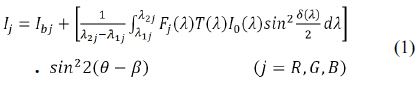
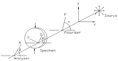
Figure 1 shows a generic plane polariscope. In dark field arrangement with white light as a source, and a color camera, the intensity of light transmitted in R, G and B sensors of the camera are given by
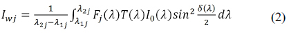
where Ibj is the intensity of the background light, I0(λ ) accounts for the amplitude of the light vector. λ1j and λ2j are the spectral limits of the light source or the camera, whichever is lower. Fj(λ ) and T(λ ) represent the spectral response of the camera and of the optical elements, respectively. δ (λ ) is the retardation, θ is the isoclinic angle of the specimen and β is the angle between the analyzer and the x-axis [1].
By letting Iwj be the intensity of the isochromatic fringe field,
Equation (1) can be written as
In the automatic polarization stepping, using a 4-step approach for isoclinic determination, a set of images with βi = I × 22.5° (i = 0, 1, 2, 3) are obtained. Eq. (3) can be written as
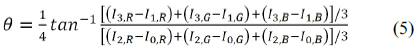
where Ii,j (i = 0, 1, 2, 3; j = R, G, B) correspond to pixel grey levels of R-, G- and B- planes for the analyzer positions of 0, 22.5°, 45° and 67.5°, respectively. The equation for evaluating the isoclinic parameter is written as [5]
Due to the fact that in white light there is no full extinction of isochromatic intensity apart from points where δ(λ )≈0, the way in which the isochromatic intensity influences the evaluation of the isoclinic is noticeably reduced.
In general, the isoclinic value θ in Eq. (5) is evaluated by atan2() function in the range of −π/4 to π/4. However, physically the true range of the isoclinic value is between −π/2 to π/2. When the physical isoclinic values are greater than π/2 or smaller than −π/2 the values obtained by atan2() function are overflowed and have abrupt jumps in the phase map, they are referred to as inconsistent zones [14]. In inconsistent zones the phase map represents the principal stress direction of the other principal stress.
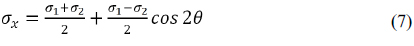
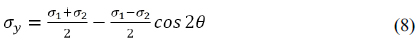
Correctly evaluating the isoclinic values is very important in photoelasticity. By using Mohr’s circle, the individual stress equations are expressed by
where σ1 and σ2 are the principal stresses, θ is the angle between the direction of σ1 and the reference axis. σx, σv and τxv are the stress components that constitute the stress tensor for a plane stress problem. In photoelasticity, the principal stress direction isoclinic is represented by the angle of σ1. If the isoclinic value is represented by the angle of σ2, by letting θ2 donates the angle of σ2, and θ2 = θ + π/2. Using Eq. (6)~Eq. (8) one obtains τxy2 = −τxy, σx2 = σy, σy2 = σx, the subscript 2 correspond to the angle θ2. Thus, the evaluated individual stress values are incorrect.
Some researchers use an approximated method to unwrap the isoclinic phase map in the range of 0 to π/2 by adding π/2 to the negative values of the isoclinic. Due to the fact that the experimentally obtained isochromatic values are always positive [1]; if the isoclinic angles θ are positive values, the shear stresses obtained by Eq. (6) are positive values only. However, the true range of shear stress values is −∞ to ∞.
To show the procedure of isoclinic phase unwrapping, the benchmark problem of a disc under diametral compression, 35 mm in diameter and 4 mm thick is used. Experimental discs are made of polycarbonate, material fringe value Fσ =7.8 N/mm/fringe, loaded of 196 N. A diffused neutral white LED light polariscope with two separate elements which can be rotated independently is setup, and an RGB camera with a resolution of 2452 × 2056 pixels is used.
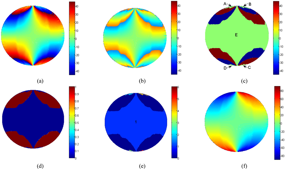
Isoclinic phase maps over the domain are calculated based on Eq. (5), Fig. 2(a) shows the wrapped isoclinic evaluated by atan2() function. As shown in Fig. 2(a), the isoclinic values suddenly shift by ±π/2 in the inconsistent zones. As long as these isoclinic values in inconsistent zones are corrected, a good unwrapped isoclinic phase map will be obtained. In order to correct the incorrect isoclinic values, one needs to identify the correctly evaluated isoclinic zones first.
In MATLAB, atan2() is a four-quadrant inverse tangent function in the range [−π, π ], and the other inverse tangent function is atan() in the range [−π/2 , π/2 ]. The wrapped isoclinic phase map evaluated by atan() function is shown in Fig. 2(b), the isoclinic value lies is in the range of −π/8 to π/8 . By comparing Fig. 2(a) with Fig. 2(b), one could find there are many regions having the same isoclinic value in two phase maps. A difference of the error term between the atan2() function evaluated isoclinic and the atan() function evaluated isoclinic is obtained; as shown in Fig. 2(c), the same isoclinic value zones are displayed in green. The data in zone E are the correctly evaluated isoclinic angle values and in this zone the isoclinic values needn’t be rectified, in zone A, B, C and D the isoclinic values represent principal stress direction of the other principal stress. The correctly evaluated isoclinic zone E has the greatest area in green zones. A threshold is applied to the error, as shown in Fig. 2(d). If the absolute value of the error is greater than the threshold the value is set to logical ‘1’, otherwise set to logical ‘0’ resulting in the modified error term. The threshold value is selected and a value of 2 is found to be suitable for most applications.
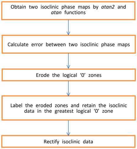
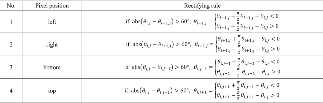
The A, B, C, D and E 5 zones are connected to each other, in order to separate 5 zones the morphological erosion [17] is performed using MATLAB V7. Erosion is a fundamental operation in morphological image processing in which the spatial form or structure of objects within an image are modified. With erosion an object in binary image shrinks uniformly. Figure 2(e) shows the eroded logical ‘0’ zones, 5 zones are completely separated. Using morphological techniques, the implementation procedure of unwrapping isoclinic is shown in the flow diagram (Fig. 3). By the labeling operation, the logical ‘0’ zones are automatically labeled as shown in Fig. 2(e). Zone E is labeled to 1 and has the greatest area and can be determined as the correctly evaluated isoclinic zones. Exclude the data in the correctly evaluated zone the rectifying process is performed within the specimen domain. The coordinates in zone 1 are used to rectify the data in Fig. 2(a). To start rectifying, a start point can be selected anywhere on the boundary of the correctly evaluated isoclinic zone. Four neighboring pixels adjacent to the selected point are rectified based on the rules [14] mentioned in Table 1. The whole field unwrapped isoclinic phase map is shown in Fig. 2(f).
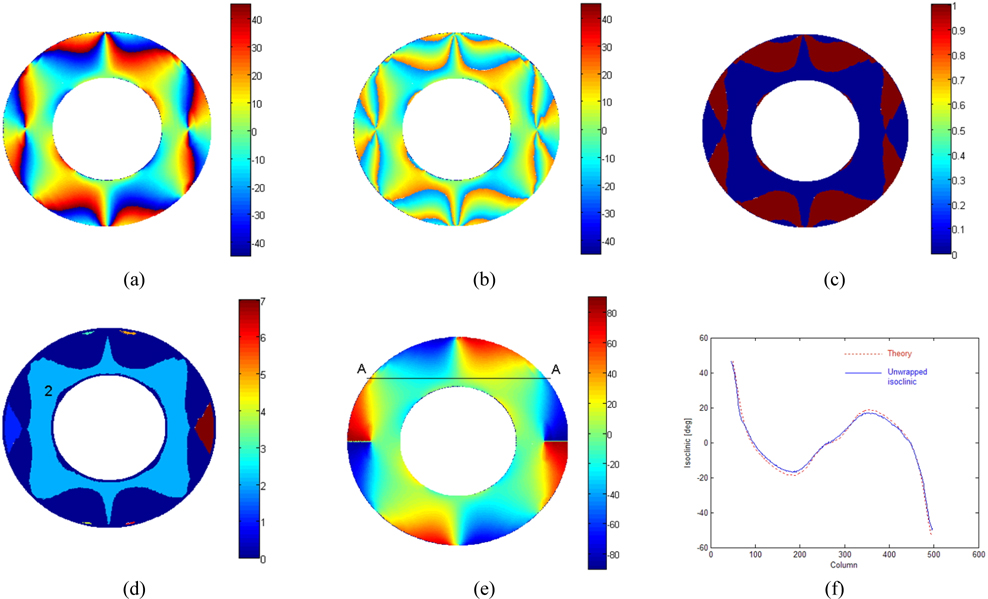
Next, the other benchmark problem of a multiply connected ring is taken up. The ring is made of polycarbonate under diametrical compression, heavily loaded of 206 N. Inner and outer diameters are 20 mm and 40 mm respectively, thickness 4 mm. Initially, isoclinic phase maps over the domain are calculated using Eq. (5). Figure 4(a) shows the wrapped isoclinic evaluated by atan2() function and Fig. 4(b) shows the wrapped isoclinic evaluated by atan() function, respectively. Figure 4(c) is the modified error after a threshold is applied to the difference error, the zones of logical ‘0’ are connected to each other. By erosion and labeling operation, the logical ‘0’ zones are separated totally, as shown in Fig. 4(d). The zone labeled to 2 has the greatest area in logical ‘0’ zones and is determined as the correctly evaluated isoclinic zone. Whole field automatically unwrapped isoclinic phase map is shown in Fig. 4(e). To verify the ability of the method quantitatively, comparison of unwrapped phase along a line A-A in Fig. 4(e) with theoretical isoclinic is shown in Fig. 4(f). The rectified results obtained using the proposed method along line A-A agree well with the theoretical results.
As known, the determination of the isoclinic parameter is not a simple task. In this paper, a new method for automatic evaluation of the isoclinic parameter is presented. The influences of principal stress direction and the range of isoclinic phase upon stress separation are discussed. It has been demonstrated that it is possible to determine the isoclinic parameter in its true phase interval of −π/2 to π/2 automatically. Using this method the ambiguity in isoclinic phase map is eliminated and the correctly demodulated regions of isoclinic phase map are retained. Furthermore, the user needn’t have a priori knowledge of the seed point to start isoclinic demodulation. Overall, the method is effective and simple for isoclinic unwrapping in white light photoelasticity, providing whole field isoclinic phase map.