Three-dimensional (3D) N-ocular imaging systems are considered a promising technology for capturing 3D information from a 3D scene [1-9]. They consist of the combination of an N-imaging system: either stereo imaging (N=2) or integral imaging (N>>2). In the well-known stereo imaging technique, two image sensors are used. On the other hand, many image sensors are used in a typical integral imaging system. Various types of 3D imaging systems have been analyzed using ray optics and diffraction optics [10-16]. Recently, a method to compare the system performance of such systems under equally-constrained resources was proposed because 3D resolution is dependent on several factors such as the number of sensors, the pixel size, and imaging optics [14,15]. Several constraints, including the number of cameras, total parallax, the total number of pixels, and the pixel size were considered in the calculation of 3D resolution, but the fact that the imaging lenses in the front of sensors produce a defocusing effect according to the object distance was ignored. In practice, this defocusing may prevent system analysis of a real N-ocular imaging system.
In this paper, we propose an improved framework for evaluating the performance of N-ocular imaging systems that takes into consideration the defocusing effect of the imaging lens in the sensor. The analysis is based on two-point-source resolution criteria using a ray projection model from image sensors. The defocusing effect according to the position of point sources is introduced to calculate the depth resolution. To show the usefulness of the proposed frame-work, Monte Carlo simulations were carried out, and the experimental results on depth resolution are presented here.
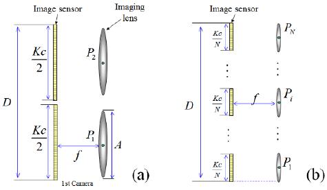
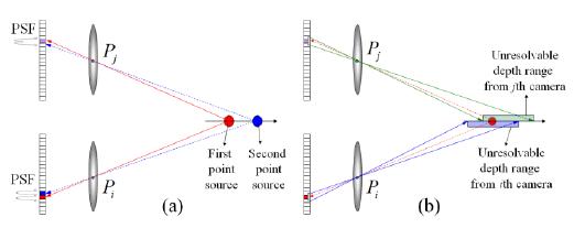
A typical N-ocular imaging system is shown in Fig. 1. Based on the value of N, the N sensors are distributed at equal intervals laterally. For objective analysis, the system design is considered to satisfy equally constrained resources. In Fig. 1, it is assumed that the total parallax (D), the pixel size (c), and the total number of pixels (K) are fixed. In addition, we assume that the diameter of the imaging lens is identical with the diameter of the sensor. Let the focal length and the diameter of the imaging lens be f and A, respectively. The number of cameras is varied from a stereo system with N=2 (2 cameras) to integral imaging with N>>2 (N cameras) under the N-ocular framework. When N=2 (stereo imaging), the conceptual design of the proposed framework is shown in Fig. 1(a) where the image sensor is composed of K/2 pixels. On the other hand, Fig. 1(b) shows an N-ocular imaging system with N cameras (known as integral imaging). Here it is composed of N cameras with K/N pixels.
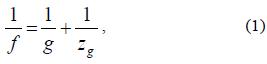
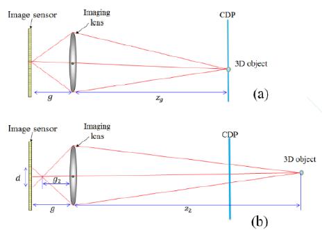
In general, the imaging lens used in the image sensor has a defocusing effect according to the distance of the 3D object, as shown in Fig. 2. We assume that the gap between the image sensor and the imaging lens is set to g. The central depth plane (CDP) is calculated by the lens formula [17].
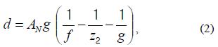
where zg is the object distance from the imaging lens. We now consider a different position (z2) of the point source outside of the CDP as shown in Fig. 2(b). From the geometry of the optical relationships and the lens formula, the diameter d for defocusing is given by [17]:
where AN is the diameter of the lens in an N-ocular imaging system and z2 is the distance of the object from the CDP.
For the N-ocular imaging system as shown in Fig. 1, we calculate the depth resolution using the proposed analysis method. To do so, we utilize two-point-source resolution criteria with spatial ray back-projection from the image sensors to the reconstruction plane. In our analysis, the diameter parameter of the defocusing effect of the imaging lens as given by Eq. (2) is newly added to the analysis process previously described in [14].
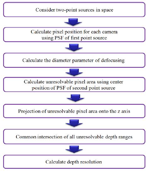
The procedure of the proposed analysis based on the resolution of two point sources is shown in Fig. 3. Firstly, we explain in detail the calculation of the depth using two point sources. This basic principle is shown in Fig. 4(a).
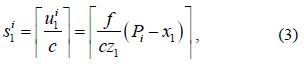
We define the depth resolution as the distance that separates two closely spaced point sources. The separation of two point sources can be calculated by separating each of their point spread functions (PSFs) independently for two adjacent sensor pixels in at leastone image sensor out of the N cameras. As shown in Fig. 4(a), two point sources are assumed to be located along the z axis. We assume that the first point source is located at (x1,z1). The first PSF of one point source is recorded by an image sensor. Note that the recorded beams are pixilated due to the discrete nature of the image sensor. The position of the recorded pixel in the sensor for the PSF of the point source is represented by
where c is the pixel size of the sensor, f is the focal length of the imaging lens, and Pi is the position of the ith imaging lens, while ⎾⏋ is the rounding operator.
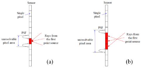
Next, we consider the second point source, as shown in Fig. 4(a). We separate the PSF of the second point source in the pixel that registered the first PSF. In this paper, we consider the defocusing effect on the position of the two point sources as given by Eq. (2). In this case, when the center of the second PSF is within the s1i pixel, the unresolvable pixel area is given by
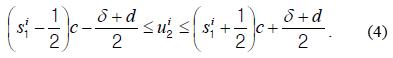
Here, δ is the size of the main lobe of the PSF, which is 1.22λf/AN. Fig. 5 shows the variation of the unresolvable pixel area according to the defocusing effect on the position of the two point sources. When the first point source is located near the CDP, the unresolvable pixel area can be calculated as shown in Fig. 5(a). On the other hand, when the first point source is away from the CDP, it is calculated as shown in Fig. 5(b). Next, we present spatial ray back-projection for all the calculated unresolvable pixel areas to calculate the depth resolution as shown in Fig. 4(b). When the ith unresolvable pixel area is back-projected onto the z axis through its corresponding imaging lens, the projected range, which we call the unresolvable depth range in space lies in the following range:
where
The unresolvable depth ranges associated with all N cameras are calculated for a given point x1. Then, the depth resolution is calculated when at least one image sensor can distinguish two point sources and can be shown to be the common intersection of all unresolvable depth ranges. Then, the depth resolution becomes
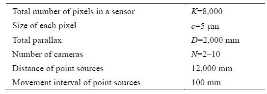
In order to statistically compute the depth resolution of Eqs. (5)–(7), we used Monte Carlo simulations. The experimental parameters are shown in Table 1. We first set the gap distance between the sensor and the imaging lens at 50.2 mm, which corresponds to a 12,000 mm CDP. The first point source is placed near the CDP. The position of the second point source is then moved randomly in the longitudinal direction to calculate the depth resolution. Under equally constrained resources, we carried out the simulation of depth resolution. The simulation is repeated for 4,000 trials with different random positions of the point sources where z (the range) is from 11,000 mm to 13,000 mm and x is varied from –100 mm to 100 mm. We averaged all calculated depth resolutions.
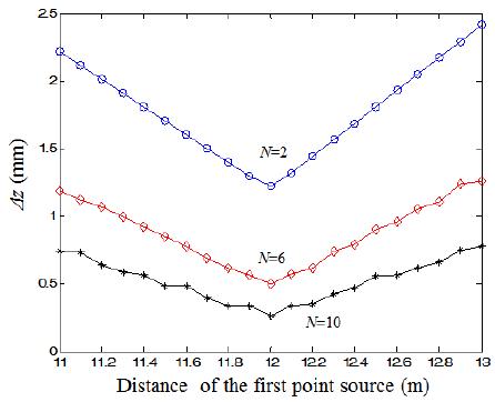
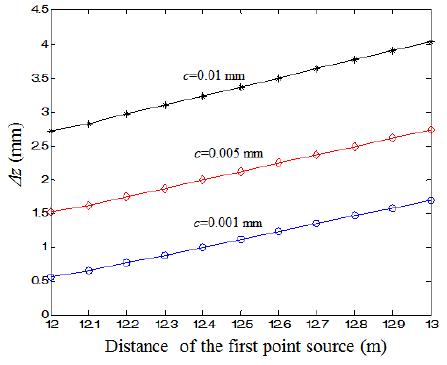
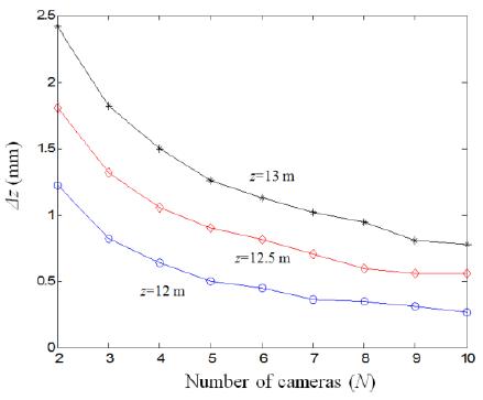
Fig. 6 shows the simulation results for depth resolution with different distances of the first point source according to the number of cameras. As the number of cameras increases, the depth resolution decreases. Fig. 7 shows the results according to the distance of the first point source.
Depth resolution is calculated by averaging the common intersection of all unresolvable depth ranges produced from N cameras. Therefore, a larger N may produce little variation, as shown in Fig. 7. Fig. 7 shows that the minimum depth resolution was obtained at z=12,000 mm because the CDP is 12,000 mm in this experiment. As the distance of the first point source moves further from the CDP, the depth resolution worsens. We also investigated the characteristics of depth resolution by changing the pixel size in the image sensors. Fig. 8 presents the results of analysis when the pixel size was varied. It was found that the depth resolution improved when the pixel size fell.
To conclude, we have presented an improved framework for analyzing N-ocular imaging systems under fixed constrained resources. The proposed analysis included the defocusing effect of the imaging lenses when calculating depth resolution. We have investigated the system performance in terms of depth resolution as a function of sensing parameters such as the number of cameras, the distance of the point sources from each other, the pixel size, and so on. Experimental results reveal that the depth resolution can be improved when the number of sensors is large and the object is located near the CDP. We expect that our improved analysis will be useful to design practical N-ocular imaging systems.