Modern container ships are characterized by large flare on the bow region for the aim to accommodate more cargo and containers. The flare region on the forward part of the hull surface experiences serious hydrodynamic load in operating conditions due to the slamming motions, which cause as result local and global damages on the hull structure. In fact, slamming has been recognized for many years as source of damage to vessels. The phenomena results when the bow region of the vessel emerges from the water and subsequently submerges at an attitude such that the angle between the water surface and the bottom plate is small creating separated water flow which will impact on the bow flare at later stage. This action induces important forces for short-time duration. Therefore it is crucial to study the water entry of ship-like sections which are arbitrary shape. Numerous studies devoted to the investigation of the water impact in theories, laboratory scale experiments, and computations.
After the study of Von Karman (1929) defined as the start of slamming research. In his work, Von Karman developed the flat plate approximation model but without considering the free surface and gravity effect. Wagner (1932) further developed von Karman’s theory by considering two fluid domains and the local elevation of water. The results are still used for the reference of impacting force in simple wedge geometry.
In case of the computational fluid dynamics, many researchers had been developed the impact simulation. The Boundary Element Method (Greenhow & Lin, 1985; Zhao & Faltinsen, 1993) based on potential flow was commonly used as a numerical solution to solve the water entry problems in the early stage of researches but this method shows drawbacks on the treatment of the water free surface and also the compressed air portion enclosed between free surface and a low dead-rise angle of section close to zero degree. Nowadays, with the improvement of computational resources and the development of robust and efficient solution algorithms (Kapsenberg, 2011), these difficulties can be surmounted by way of Computational Fluid Dynamics (CFD) methods. In fact, CFD methods have been applied to impact problems for the two last decades for many aims in particular to predict local pressures on the bottom surface using the Navier-Stokes solver and VOF transport method (Ochi & Motter, 1973; Yum & Yoon, 2008), and investigated gravity and momentum effects during water entry (Fairlie-Clarke & Tveitnes, 2008), and free surface motions with floating structures by Moving Particle Semi-implicit (MPS) (Lee, et al., 2008), and air compressibility effect of the water impact (Phi & Ahn, 2011).
In almost of the aforementioned studies, the model that used in the simulation is either simple wedge or Zhao model (Zhao & Faltinsen, 1993) whose shape does not have bulb. In the present study, a commercial CFD code ANSYS FLUENT® (ANSYS Fluent user’s guide, 2015) is used to simulate two cases: one is to validate impact pressure using conventionally well-known test case by Zhao et al. (Zhao & Faltinsen, 1993), second is two different bow flare sections with constant velocities in order to investigate the effect of velocity variation during water entry and predict the pressure history for different flares with the influence of bulbous bow section shapes: Panamax-like(with small convex bulb and flare) and Post panamax-like(with large convex bulb and flare).
2. Summary of Fluent numerical method
We refer a short summary of the Fluent simulation function what we had been used. ANSYS FLUENT® uses a control-volume-based technique to convert the governing equations into algebraic equations that can be solved numerically; the governing equations are integrated in each control volume and discretized to conserve each quantity of mass and momentum on a control-volume basis.
The pressure-based segregated algorithm is employed to reach a conversed numerical solution of the governing equations through the “Semi-Implicit Method for Pressure Linked Equations” scheme. SIMPLE solves the equations sequentially and uses a relationship between velocity and pressure corrections to enforce mass conservation and to obtain the pressure field. The spatial discretization is based on the Second-Order Upwind scheme which uses larger stencils for second order accuracy, essential with triangle-mesh and when flow is not aligned with grid.
The flow is considered as turbulent and viscous effects is included in present analyses by integrating the standard k-ε turbulence model which is a semi-empirical model, therefore, the governing equations to be solved are the continuity equation, the Reynolds averaged Navier-Stokes(RANS) equation and the model transport equations for the turbulence kinetic energy (k) and its dissipation rate (ε).
The free surface is modeled by Volume of Fluid (VOF) method. The VOF method assigns a variable for each fluid indicating what fraction of that particular fluid is in the cell and the total of these variables for all fluids sums up to unity in every cell. The fluids share a single set of momentum equations and the volume fraction of each fluid is tracked throughout the domain. The fluid properties in a cell are dependent on the volume fractions of the fluid within it. The free surface occurs at cells that have volume fractions of one half for each of the two adjacent fluids. For this matter, different explicit and implicit discretization schemes for interpolation near the free surface are provided by ANSYS FLUENT®. In present analysis, time-dependent explicit Geometric Reconstruction interpolation (Geo-Reconstruct) scheme is used. Geo-Reconstruct is the most accurate scheme offered by the current CFD solver ANSYS Fluent user’s guide, 2015)
3. Validation of flare section drop test
3.1 MARINTEK Experiments (
In this section, the RANS based solver FLUENT® is validated with the drop test carried out by Zhao et al. in 1996 at MARINTEK. Details of the experiment are described in reference (Zhao, et al., 1996).
[Table 1] Detail of section drop test setup
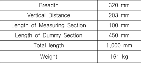
Detail of section drop test setup
3.2 Boundary conditions and fluid properties
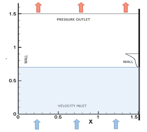
In this simulation, the arbitrary flare section is kept stationary while the flow originated from the inlet flowed upward with an imposed velocity inlet on the bottom. At the top of the domain, a pressure boundary condition set at atmospheric pressure is imposed in order to evacuate the excess of air in the domain. The arbitrary flare section geometry and the domain walls are defined as slip wall boundary condition. For the interface boundary condition, pressure is constant across the free surface interface on atmosphere p=, and it follows the transportation equation of mass of volume of fluid. The water inside domain is considered as incompressible with a density equal to 998.2 kg/m3, air density is equal to 1.293 kg/m3.
3.3 Domain and mesh parameters
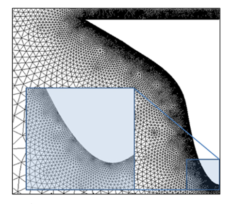
The computational domain’s size is 3.0 m × 1.5 m as shown in the Fig. 2(for the simplicity, it shows the half). The mesh is a surface all triangular type meshes patched independently and composed of 110,576 cells, 57,042 nodes and 167,618 faces. The maximum size of the curved mesh along the body surface of the geometrical section is equal to 0.0005 m. The initial position of free surface is set by the horizontal line coinciding with the bottom of the arbitrary flare section at an elevation equal to 0.7 m.
3.4 Water entry velocity variations
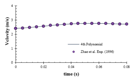
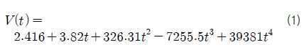
In real drop test case, the impact velocity varies during the water penetration period according to the mass of the section and its geometrical shape. The experimental entry velocity profile of the arbitrary flare section is shown in the Fig. 4 and initialized with a velocity equal to 2.416 m/s which is the same as the experiments. The total impact period recorded for the experiment is 0.08 seconds.
To adapt the velocity variations during the numerical simulation, it is necessary to know the experimental impact velocity profile in order to express it numerically. In the present study, accelerated effect is integrated during the simulation by way of an UDF imposing an inlet velocity which is interpolated by the experimental velocity with regards of time in Eq. (1). Numerical velocity will be updated every time step according to a forth order polynomial introduced as a DEFINE_PROFILE macro in the UDF (ANSYS fluent UDF Manual, 2015).
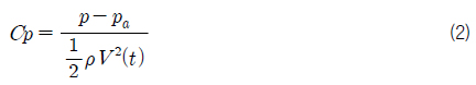
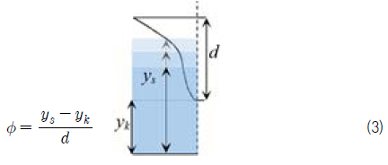
All computations in this paper using FLUENT satisfied the mass conservation within the order of 10−3 and time step is 5×10⁻⁵(s). Results are evaluated based on dimensionless parameters: the pressure coefficient expressed in terms of entry velocity and density, and the non-dimensional depth expressed based on the section draft.
The pressure coefficient (Cp):

where
The non-dimensional depth (

where
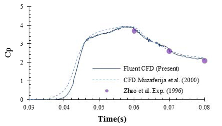
The aim of the numerical simulation is to record the time pressure history of local pressure at two specific points localized on non-dimensional depth levels equal to
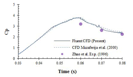
The results present in Fig. 5 and Fig. 6 present the time history of local pressure at
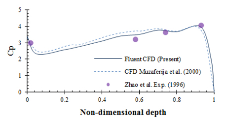
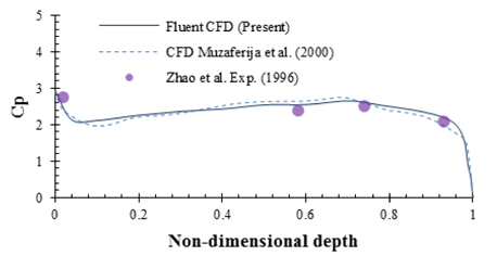
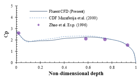
Fig. 7, Fig. 8 and Fig. 9 show the pressure distributions along the arbitrary flare section at t=0.06 s, t=0.07 s and t=0.08 s respectively from the initial contact of the arbitrary flare section with the free surface. The non-dimensional depth on the level of the section keel is equal
4. Numerical study on local impact pressure on different bow flare sections
The results discussed in the previous section show a satisfactory agreement with the experimental results of Zhao, et al. (1996). The previous section demonstrated as well the robust reliability of the commercial CFD code ANSYS FLUENT® which is based on solving Navier-Stokes equations, and a good accuracy on the pressure prediction and monitoring.
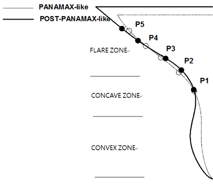
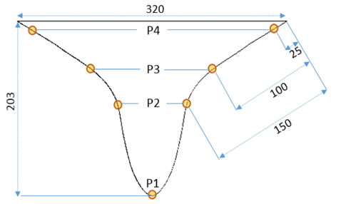
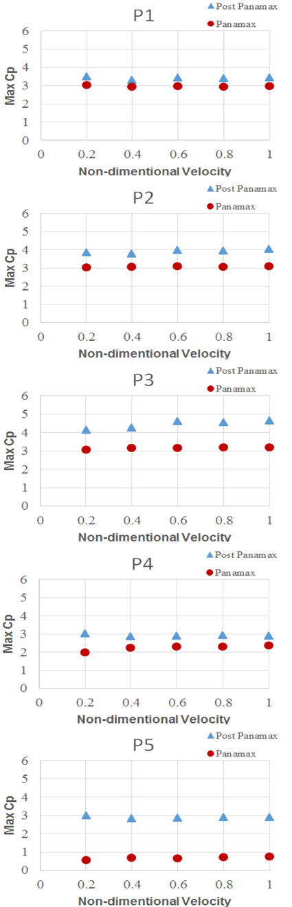
In this section, we propose to simulate numerically drop tests of panamax-like(PANA hereafter) and post-panamax-like (POSTPANA hereafter) bow flare sections under different conditions in order to investigate on the effects of water entry velocity, bulb region shape, flare angle and the pressure impact in the both cases. The PANA(small convexed bulb) and POSTPANA(large convexed bulb) refer and scale down from Matsunami (2004), and placed five points(P1 through P5) to monitor pressure values which is developed during the water impact. As shown in Fig. 10, the five points locate in the concave zone and flare zone.
4.1 Vessel section-like drop tests
Drop tests have been numerically simulated with two arbitrary bow flare sections, a panamax-like section(with small convex bulb) and a post-panamax-like section(with large convex bulb) as described on the Fig. 10. The panamax-like section shows a straight shaped bulb on the bottom part with low angled concave shape flare, whereas high concave shaped flare angle with convex shaped bulb are present in the post-panamax-like section. In the shape, there are three zones: convex zone in bulb region, concave zone, and flare zone.
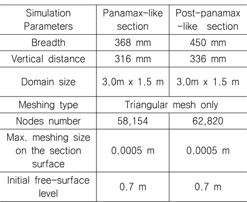
Numerical simulations have been carried out under different constant velocities 2, 4, 6, 8 and 10m/s for both bow sections cases. In all simulations, local pressure was recorded in 5 measurement pressure points P1, P2, P3, P4 and P5 located on the section’s body surface at different levels as shown in the Fig. 10. Simulation parameters for the drop tests in Table 2 are same as the settings described in the previous section 3.
[Table 2] Drop tests domain and meshing parameters

Drop tests domain and meshing parameters
The maximum pressure values measured in each point during section water entry were simulated. With given five points to be monitored shown in Fig. 10, maximum pressure coefficient values (Cp) measured in every measurement point after drop tests with different water entry velocities for both bow flare sections summarized along non-dimensional velocity by maximum drop velocity of 10m/s is shown in Fig. 11. The calculation results show that the Cp value of the POSTPANA case in all the drop velocity has bigger than that of the PANA case. Going through the P1, P2 and P3, the difference of Maximum Cp between PANA and POSTPANA has increased. The difference at P4 is small again, and the biggest difference shown at P5. It is due to the dead-rise angle at the measuring point. Comparing to the PANA bow section, it is clear that the POSTPANA bow section experiences higher pressure during the water entry with the same velocity due to its more concave shape and larger flare. Fig 11 is also shown that both PANA and POSTPANA are followed the relation of the pressure and drop speed to be squared according to the various speeds. However, POSTPANA case does not follow the relations as much as PANA case because the large curved bow shape and large flare angle.
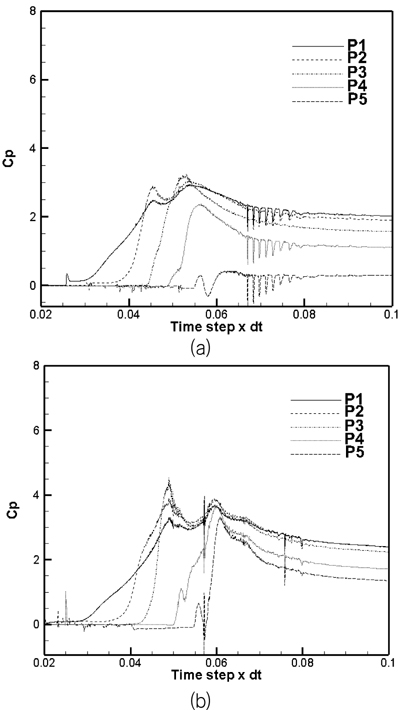
In order to see the coefficient of pressure development with time, a typical Cp pattern is elucidated in Fig. 12 at 4 m/s. The pattern is almost same through the different drop velocity. The Cp pattern of the arbitrary shape with bulb shows a tendency of two picks at the impact velocity due to the convex shape. The pattern is different with the Cp on the plate wedge case having only one pick pattern at the constant velocity in the Fluent simulation (Yum & Yoon 2008). The second pick has shown in the POSTPANA strongly than PANA case. Impact pressure on the points where locate in the concave zone has been affected by the forementioned convexed bulb shape. In case of P3 both PANA and POSTPANA, P3 in PANA has one-pick monotonic pattern while P3 in POSTPANA has two-pick pattern. Simulation shows that first impact Cp on P1, P2, and P3 in POSTPANA has almost the same time step of 0.049. It is due to the large dead-rise angle on P3 along the five points. Around the second pick time step of 0.0555, both P4 and P5 participate the impact Cp. as the pressure pattern of the simple wedge which small dead-rise angle has bigger value of the pressure. After the impact, the Cp values approach its total pressure including static pressure and dynamic pressure.
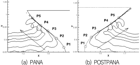
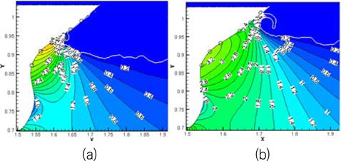
In Fig. 13, free surface development by FLUENT volume of fluid field shows from 0.042 to 0.055 time step. Those steps are between the two picks shown by both PANA and POSTPANA. The free surface pattern includes a lump of water near the solid shape as well as sharp water splash along the solid surface over the viscosity region. The visualization shows that thin free surface layer forms at early stage of the impact. The free surface pattern also shows that POSTPANA free surface has more scroll down due to the larger dead-rise angle than PANA case.
[Fig. 13] velocity (a) PANA and (b) POSTPANA (0.037, 0.042, 0.048, 0.05, 0.0525 and 0.055 time step)

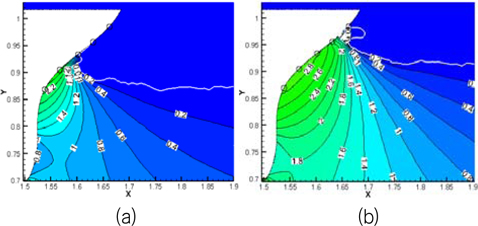
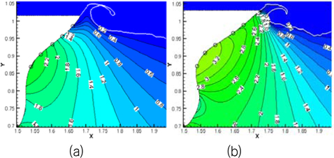
In order to elucidate the Cp curve pattern in the arbitrary shape, we plot Cp field from 0.0 to 5.0 calculated on the total pressure. The interval of Cp value is 0.2 and white line denote free surface at specific time step. In Fig. 14, PANA in constant drop velocity 4m/s shows at the time step of 0.045 and 0.055. At 0.045 in Fig. 14(a), P1 and P2 have start to impact and P3 participates at 0.055 time step in Fig. 14(b). In case of POSTPANA having the large flare, Cp graph shows more steep and sharp pattern. In Fig. 15(a), it shows dense contour lines in the center of P3 at 0.049 time step for the first impact while at 0.0555 for the second impact, it did not show any type of impact-focusing to the points. The pressure spreads out through the concave and flare zone.
In case of pressure value on P5 where is the nearest to deck, it is significantly different between PANA and POSTPANA in Fig. 16. It is because that the dead-rise angle in PANA is larger than POSTPANA, and the difference also comes from the previous dead-rise angle on P4 which is comparatively smaller than P5 in PANA. POSTPANA in Fig. 16(b) having the relatively small dead-rise angle remains high pressure around corner.
We summarized that POSTPANA with big bulb and large flare than the PANA’s one suffers large impact pressure. At given impact velocity, the big bulb makes the several pressure picks at different places could be gathered at a moment and large flare also has bigger pressure on the arbitrary surface according to the simulation results.
We carried out two-dimensional water impact simulation by two different arbitrary bulbous-like shapes by using A commercial Reynolds averaged Navier-Stokes based solver FLUENT® to investigate the water entry impact of two-dimensional arbitrary solid bow flare sections.
The numerical results obtained by Fluent were validated with drop test by Zhao, et al. (1996) and showed a satisfactory agreement with the experimental data. For the two arbitrary ship bow sections panamax-like(with small convexbulb region) and post panamax-like(with large convexbulb region) under the constant given entry velocities from 2 m/s to 10 m/s.
Simulation results on the bulbous arbitrary shape show two different aspects comparing with the conventional simple wedge. One is that pressure coefficient is possible to have double picks and the other is that the maximum pressure values happen at the same time even the place is different. It is due to the two types of flow tracked by the solid impact consist of thin layer in the viscosity region and a lump of water on the vicinity of solid-free surface. In the simulation results, the lumped water before the form of a splash is a role of capturing momentum energy. After generating the splash, the captured effect seems to be vanished. Though the lumped water exists both panama-like and post-panama like, the Post-panama like bulb has more influence on the impact pressure with its lower angled flare than that of Panama case. Finally, we conclude that the bulb-type arbitrary shape follows an amount of the lumped water during its entry, and the impact pick happens in a close time simultaneously in the simulation which can be harmful to the solid surface.