Bioinformatics is the convergence of diverse and often divergent fields such as biology, mathematics, statistics, computer science, and computer engineering. Bioinformatics seeks to find answers to the all-relevant and all-important question of the origin of life and the processes of life. Bioinformatics takes a different perspective on life depending on the scale or scope on which life is considered. From the perspectives varying from molecular to organism to evolution, one process lies at the heart of it all: sequence alignment.
Sequence alignment is concerned with finding the relatedness of one sequence to another sequence. Relatedness indicates whether the sequences are homologous and whether they share a common domain and motifs or not. Finding relationships among biological sequences helps significantly in knowing concepts such as how proteins are related to each other in an organism and to other organisms with which this organism shares an evolutionary history, thus providing significant insight into the meaning and function of life. Moreover, sequence alignment has diverse applications such as drug engineering, disease diagnostics, detection of autoimmune disease, genetic engineering of plants and animals, determination of the structure of proteins, evolution tracing, and determination of protein functions [1]. Sequence alignment compares two sequences by calculating the distance between the sequences. This distance represents the minimal cost at which one sequence can be converted into another. A score is assigned to each distance computed, and from this distance matrix, the degree of similarity or correlation between the sequences is inferred. For computing the abovementioned distance, two elementary operations are used, namely substitution and insertion/deletion (indel). Substitution signifies that one base in the sequence is replaced by another, while indel represents the insertion/deletion of a base into/from the sequence.
DNA is composed of four bases, namely adenine, cytosine, thymine, and guanine. When aligning two sequences, these bases are represented by the letters A, C, T, and G, respectively. Strings of these letters form a DNA sequence. Further, the basic alignment tool is the dot matrix. In this type of alignment, one sequence is arranged row-wise, while the other is arranged column-wise. A dot is placed in the cell that corresponds to a match of the letters of the row and the column.
As can be seen, DNA sequence alignment can be a very tedious and resource-intensive operation because DNA sequences can be millions of characters long and aligning them by conventional methods is not possible. For the alignment process to be meaningful, it needs to be accelerated. Such acceleration can be carried by using either software or hardware. Software acceleration employs heuristic methods and hence, is not optimal. For optimal acceleration, exact methods that compare each character against every character of the other sequence are required. Exact methods are very time consuming and resource intensive. To achieve optimality, they need to be carried out on dedicated hardware.
The Smith–Waterman algorithm (SWA) is an exact sequence matching algorithm that performs optimally as it can return local alignments and thus, provide considerably accurate information about the similarity between sequences that are aligned against each other [2]. SWA is a dynamic programming-based algorithm that decomposes the alignment problem into sub-problems and iteratively solves the given problem [3]. SWA has the space and time complexity of
SWA is a resource-intensive operation and thus, needs dedicated hardware for efficient and fast operation. Different hardware implementation candidates can be found, such as FPGA, GPU, and cell BE platforms. In [4], a comparison between the FPGA, GPU, and cell BE reconfigurable platforms for aligning biological sequences on the basis of speed, energy consumption, and developmental costs has been presented. Further, it has reported that FPGA outperforms the other two platforms in terms of performance per watt and performance per dollar spent. The advantage of FPGA in high-performance computing is that, if it is used as an accelerator, the computing density can be increased significantly as FPGA benefits from the increased clock speed as opposed to general microprocessors that have reached their maximum clock speed [5].
Because of the low cost and speed-related advantages, all recent hardware-based SWA implementations are carried out on FPGAs [6]. The performance of an implementation on FPGA depends upon the cell design that does the calculation for SWA. This work focuses on designing an efficient systolic cell for implementing SWA on FPGA. The main objective of this work is to design a systolic cell that uses relatively few hardware resources but at the same time, is not designed on a low-level device/platform and does not depend on the specific details of the low-level device/platform. Therefore, the design can be implemented on any other FPGA device or platform. Our implementation has a trade-off between complexity and performance. Moreover, it avoids both oversimplification and wastage of hardware resources by avoiding a direct mapping of the iterative equations to the hardware. This work should be considered in a broader framework developed by [7] and focuses particularly on designing a cell that optimally fits the system design of [7].
The performance issues associated with the transfer of the required data to FPGA and back has been studied by [8]. GPU platforms are explored in the same capacity as FPGA. The authors in [9] studied the well-known seed-and-extend algorithm to accelerate sequence alignment. Meaningful alignment often requires the alignment of short DNA sequences. The mechanisms and specifics of the alignment of short DNA sequences are sometimes divergent with the goals of the alignment of large sequences. The authors in [10] developed a platform that through GPU could accelerate the alignment of short sequences. Other architectures are also explored for accelerating the alignment of DNA sequences. In [11], a single instruction multiple data (SIMD)-based architecture is implemented on an application-specific instruction-set processor (ASIP) for aligning DNA sequences.
The rest of this paper is organized as follows: Section II discusses the SWA in detail. Section III presents the principles on which the proposed cell design is based. Section IV describes the proposed cell design. Section V presents the results of this study, and Section VI concludes the paper.
Needleman–Wunch [12] presented an efficient algorithm(NW algorithm) for aligning two sequences. The method was exact and thus, produced optimal results. However, it performed global alignments. Global alignments are good when the sequences to be aligned are closely related as end-to-end alignment highlights the similarity across their lengths but they fail to perform optimally when the sequences to be aligned do not have large homology. Smith and Waterman presented a variant of the NW algorithm in 1984 and called it the Smith–Waterman algorithm (SWA) [3]. SWA finds the local alignment and works well for sequences that are distantly related as such sequences do not manifest the overall similarity but have regions that have concentrated local similarities.
Local alignments are carried out by making small changes to the equations that perform global alignments. SWA like the NW algorithm consists of three stages for performing alignment, namely initialization, matrix fill, and trace back. The initialization and matrix fill stages resemble those of the NW algorithm, while the trace back stage differs from that of the NW algorithm. These three stages can be described as follows:
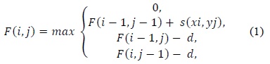
(1) uses a linear gap penalty scheme as every gap is penalized in the same way. A more biologically relevant method for handling gaps is the affine gap model that penalizes opening a gap more than extending an already opened gap. Such a scheme is given in (2).


In (3) and (4),
Before presenting the system model, we will evaluate the performance of the SWA used in the proposed design.
>
A. Performance Evaluation of SWA
SWA performs optimally on many performance indicators such as accuracy, parallelism, and space and time complexity [13]. SWA is considered the most optimal because it performs the alignment of every individual character in one sequence against every character in the other sequence. This results in the massive space complexity of
Both fine-grained and coarse-grained parallelism can be exploited in SWA. Fine-grained parallelism works on making the required data available for a cell and then computing the values of these cells in parallel; the values of the three previous cells are available for this computation. Coarse-grained parallelism is achieved by dividing the alignment problem into sub-problems and solving the sub-problems in parallel, thus reducing the overall time complexity.
In calculations that are not parallel, computing the entire matrix takes
>
B. Systolic Cell Design for SWA
This section presents an efficient PE design for aligning two sequences by using a linear systolic array (LSA) on FPGA. The systolic array was introduced by Kung and Leiserson [15]. Systolic arrays have proven to be significantly efficient in parallelizing computing designs. These arrays have been used for performing the complex function of multiplying two long sequences: the sequences are arranged in rows and columns, and two elements from the sequences are multiplied by the PE in a systolic array. The idea of systolic arrays was used by Lipton and Lopresti [16] in 1985 for implementing the edit distance algorithm, a standard global alignment algorithm for DNA sequences. In 1987, on the basis of the initial results, which showed an improvement in speed in the order of hundreds to thousands of times, Lopresti developed the first full-fledged system for aligning nucleic sequences. This system was called P-NAC. Further, BISP, Bio-Scan, B-Sys, Splash/Splash 2, and Kestrel employ systolic arrays for aligning two sequences.
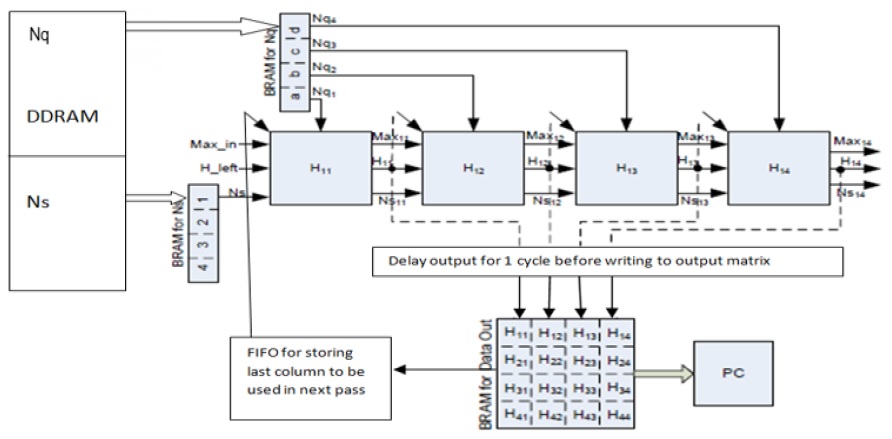
When SWA is mapped to a systolic array, each PE computes one element of the alignment matrix at a time, and an entire column is computed during the time span of the entire operation. Further a PE array is mapped to the anti-diagonal lines of the alignment matrix. A PE that is composed of elements that perform simple operations such as addition, subtraction, and comparison makes the design very fast. The focus is always on making the PE simpler, faster, and thus, more efficient. The overall system design is adopted from our previous work as presented in [7]; the corresponding block diagram is illustrated in Fig. 1.
To achieve the goal of designing an efficient PE, it is imperative to reduce the area that a PE uses. Besides being slow, oversized PEs waste significant hardware resources. This reduces the available resources that can be used for realizing a large number of PEs and hence, reducing the size of the LSA. The size of the LSA controls the degree of parallelism and thus, the speed-up achieved. Oversized PE also adversely affects the clock frequency through which the LSA operates. As the number of logic units increases in a PE, the clock will need more time to traverse to the end, subsequently affecting the rate at which the computation of the PE can be completed.
Previous design methods of PE can be broadly categorized into three categories: The first one oversimplifies the design of PE. The second approach employs a direct implementation of an iterative equation to the LSA. The third approach attempts to carry out optimizations at the VLSI level by integrating two PEs. All these approaches have problems of their own. The first method calculates only the edit distance between two sequences and thus, results in non-used hardware resources. The second results in an overuse of hardware resources, while the third results in compatibility issues as such a design cannot be migrated to other platforms.
Therefore, we need to come up with a design that avoids all of the abovementioned pitfalls. A design which is not overly-simplified and does not overuse resources, and which is also compatible with other platforms is needed. The next section looks at such a design for aligning two sequences by using SWA with linear gap penalties.
This section presents the proposed design for SWA. First, the cell design for SWA with a linear gap penalty is presented, and then, the cell design for SWA with an affine gap penalty is discussed.
>
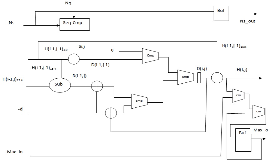
A. PE Design for SWA with Linear Gap Penalty
A portable design that judiciously uses hardware is possible if the iterative equations of SWA can be simplified and captured in standard hardware description languages (HDLs) such as Verilog. The major bottleneck with the recursive equation of SWA is that the data precision of the computed elements is very high. For the alignment of DNA sequences, a data precision of 16 bits is used. The logic units that a PE uses are very basic, such as adders and comparators, but the size of these units increases the hardware resources consumed by an individual PE. Therefore, the size of the logic units needs to be reduced to achieve an overall improvement in the hardware utilization. If Lopresti’s observation is realized in the field of PE design, significant savings in hardware usage can be achieved.
In 1985, Lipton and Lopresti [16] observed that the values of the top element
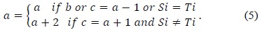
In (5),


The values as computed in (6) and (7) are used as intermediate values, and thus, the adders and comparators involved compare two inputs of two bits each instead of two inputs of 16 bits each. The output
>
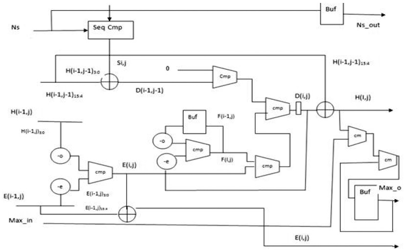
B. PE Design for SWA with Affine Gap Penalty
Affine gap models are used for aptly representing the biological fact of the costliness of opening a gap than that of extending it. An affine gap model penalizes opening a gap more than extending an already opened one. (2)–(4) present the Smith–Waterman iterative equations for affine gap models. Fig. 3 presents the block diagram for an affine gap penalty cell.
Two new units are added to calculate
In order to reduce the cost incurred by acceleration through FPGA, we implemented the design on low-cost Spartan-3 FPGA, a product of Xilinx. Spartan-3 is a low-priced device of Xilinx but is sufficient for implementing a design of low–mid-level complexity. It does not contain many logic slices to realize a high-performance design. It does not allow the implementation of PEs in the order of hundreds. The implementation of only a limited number of PEs is allowed. This affects the overall speed-up achieved. The speed-up achieved is at a cost incurred such as energy consumption and hardware resources used, thus, a balance has to be maintained between speed-up achieved and the cost incurred.
The most often used performance metric for computational biology applications is the number of cells updated per second (CUPS), and it can be calculated as expressed in(8):

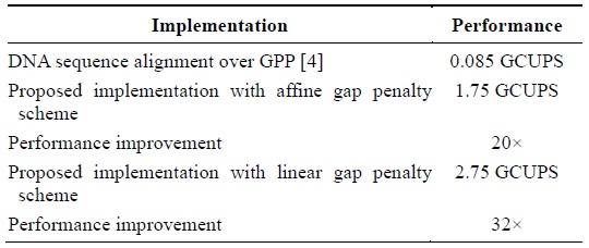
The device that we used is Spartan 3 XC3S250E. We could instantiate an array of PEs of size 35 on the said device. The operating frequency shown by the post-place and route simulation model was 50 MHz. The proposed cell design implemented in the framework results in 1.75 GCUPS for the affine gap penalty cell and 2.75 for the linear gap penalty cell. This is a 20× and 32× performance improvement over the GPP implementation described in [4]. Table 1 presents the performance improvement.
[Table 1.] Performance improvement in terms of CUPS

Performance improvement in terms of CUPS
The authors of [17] built highly customizable PEs for the alignment of biological sequences on FPGA. They could implement an array of PEs of size 13 on a Spartan 3 1500 chip. Table 2 presents the efficiency of the proposed design in terms of the hardware utilization. The proposed design more efficiently utilizes hardware as it can realize more PEs by using limited hardware resources in contrast to the implementation described in [5] that realized fewer PEs by using a lot of the hardware resources available.
[Table 2.] Hardware utilization improvement
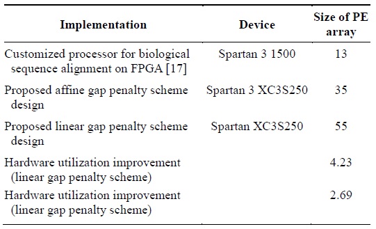
Hardware utilization improvement
The number of PEs realized can be increased if our memory utilization logic is not implemented and an UART that directly sends the output is used. Performance can be improved by using a device that has a higher clock speed and has more hardware resources available.
Implement-ations such as the implementation described in [18] achieve very high performance but at a very high cost; further, the design cannot be implemented on any other platform because it incorporates the VLSI-level details as in contrast, the proposed system achieves comparable per-formance at a very low cost.
In this paper, we presented an efficient and low-hardware-resource-consuming systolic cell design for implementing SWA on FPGA. Cell design is the most important part of designing an efficient and fast implementation of SWA on FPGA because the actual matching takes place here. Previous designs either oversimplified the cell design for implementing the iterative equations or avoided optimization altogether and directly mapped the iterative equations to the hardware. This resulted in either inflexibility or the wastage of hardware resources.
The proposed design aimed at a trade-off between flexibility and performance. Equivalent equations of the iterative equations that require fewer iterations for the implementation were used instead of the original iterative equations. The results showed performance improvement over a GPP implementation in the order of 32× for the linear gap penalty scheme and of 20× for the affine gap penalty scheme. Moreover, the results were compared with those of a design that was implemented on a device that had more hardware resources than our Spartan XC3S250. Further, we showed that the proposed design surpassed the hardware resource utilization of the other design by a factor of 4.29 in the case of the linear gap penalty scheme.