Multi-input multi-output (MIMO) technology is widely considered to be a promising solution for telecommunication systems because of its many advantages. However, as mobile devices continue to become smaller because of the limitations of space and crosstalk (overlapping), the complexity of designing a multi-antenna system for use in compact devices increases. Among the approaches suggested for solving this problem, the characteristic mode analysis (CMA) is preferred because of its usefulness in intuitively understanding the antenna itself.
CMA is a theory of field analysis, which can describe the surface current in an arbitrary structure in terms of eigencurrents known as characteristic currents [1,2]. The far-field produced by each eigencurrent is orthogonal, and thus it can be used to determine the appropriate position for antennas when designing MIMO systems. Various approaches have been proposed to take advantage of the characteristic mode.
In [3], a systematic antenna placement procedure was demonstrated using CMA and the bandwidth potential concept. In [4], the position of dual antennas in a mobile terminal was determined based on CMA below the 1 GHz band. Further, in [5], a practical coupling structural concept, the Booster, was introduced to use CMA in a MIMO antenna design. [6] proposed the coupling structure for the current correlation coupling to be an exciter.
In this work, we propose the use of the factor known as the current correlation coefficient (
CMA was proposed and generalized by Garbacz and Turpin [1] and Harrington and Mautz [2]. After solving the method of moments (MoM), we obtain the Z-matrix, which is then decomposed into the eigenvalue and the eigenvector (eigenfunction or characteristic current). Solving the equation [
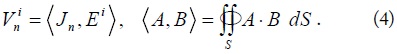
Assuming the E-field

Physically,

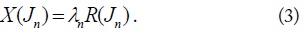
where

In Eq. (3),
The modal coefficient can also be derived, assuming that the total current is expressed by a linear combination of the characteristic currents. Therefore,

Applying all the above mentioned results, we can express the total current as follows:
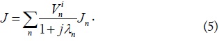
The physical meaning of Eq. (5) is that the total current
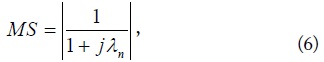
which denotes how well the mode radiates at a particular frequency. As the MS increases to 1, the mode radiates more efficiently.
In practical terms, we require an additional structure to use the specific mode we desire. Two potential approaches are available. First, the mobile terminal itself can be used as an antenna with an electrically small coupling structure called the Booster. The second approach involves adding an antenna onto the ground plane. In the second case, we need to focus on the coupling problem,
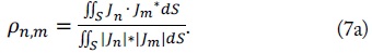
To make better use of CMA in the design process for MIMO systems, we propose a practical parameter called

Then, it is discretized as follows:
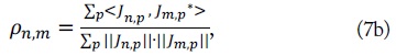
where each
Therefore, we can use
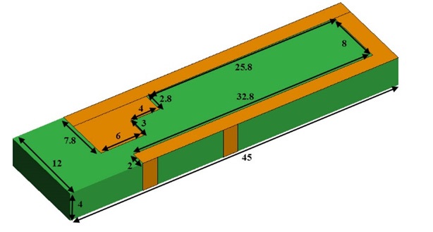
The size of the ground structure is 134 mm × 79 mm, and it is composed of PEC and FR4 (
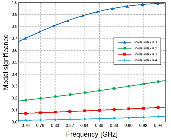
Considering the eigenvalues (Fig. 3) of each mode of the structure, we choose mode 1, which has a higher MS than the other modes. Therefore, mode 1 is the most efficient mode below 1 GHz. Mode 1 has a longitudinal current distribution shape. With this structure and
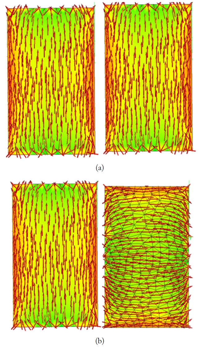
The Booster is an electrically small coupler used to excite the specific mode we desire. It has a relatively small size compared with the structure. Therefore, whether it is attached or not, no significant change is observed in the characteristic current distribution of the structure (Fig. 4). When the Booster structure is placed in the correct position, we can excite the mode we targeted without disturbing its own characteristic current distribution.
Among all the proposed structures, we choose a simple cuboid structure [5] to verify the usefulness of the
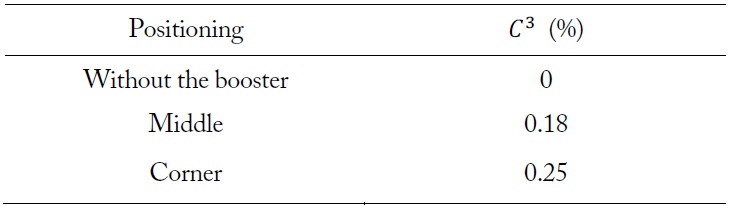
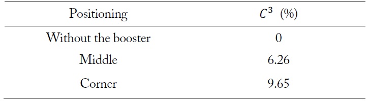
To validate this method, we change the position of the Booster along the short edge of the ground plane and then check the
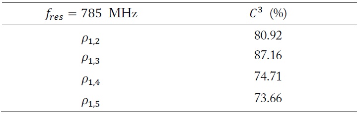
[Table 1.] Current correlation coefficient (C3) values according to the position change (see Fig. 4)

Current correlation coefficient (C3) values according to the position change (see Fig. 4)
2. The Radiator Placement Case
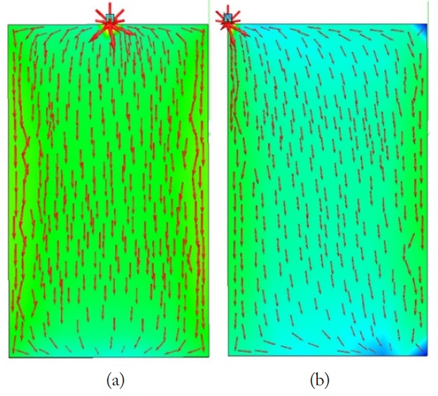
The radiator has its own radiating structure without a ground plane. We use the same procedure (Fig. 5) to observe the
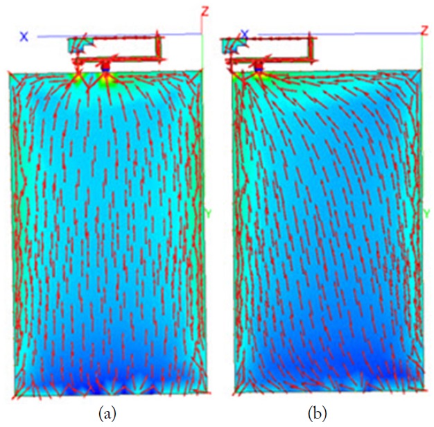
[Fig. 5.] Current distribution depending on the position of the radiator: (a) middle and (b) corner.
[Table 2.] Current correlation coefficient (C3) values according to the position change (see Fig. 5)

Current correlation coefficient (C3) values according to the position change (see Fig. 5)
The results indicate that the degree of freedom of the design can be reduced when we use a radiating structure to excite the mode we want.
CMA appears to lose its advantage when the structure is modified because the outcome of the analysis can also be changed. Thus, using the radiator as a coupler for the specific mode can be disadvantageous in the design process.
The radiator can be affected by the ground plane and also by other radiators. Using
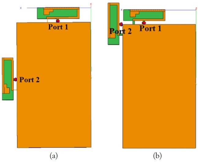
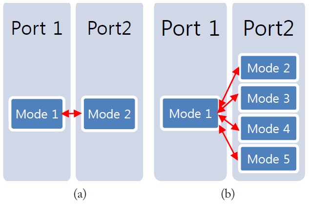
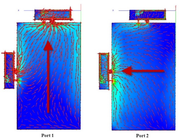
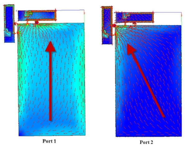
When considering the coupling between several antennas mounted on the same ground plane,
According to the results (Tables 3 and 4), a correlation is observed between ports 1 and 2 of the Corner model. The Middle model has a relatively smaller amount of correlation current distribution produced by ports 1 and 2 than the Corner model. (Tables 3 and 4) present the current correlation between the characteristic currents. The Middle model has a relatively smaller
[Table 3.] Current correlation coefficient (C3) value of the Middle model (see Fig. 8(a))
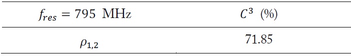
Current correlation coefficient (C3) value of the Middle model (see Fig. 8(a))
[Table 4.] Current correlation coefficient (C3) values of the Corner model (see Fig. 8(b))

Current correlation coefficient (C3) values of the Corner model (see Fig. 8(b))
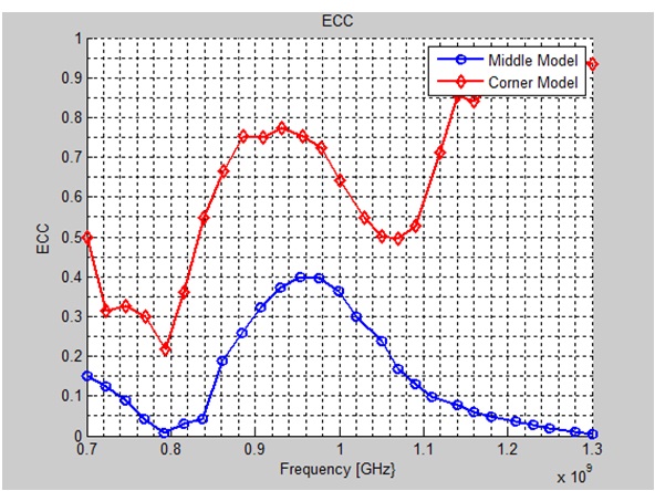
The envelope correlation coefficient (ECC) is the parameter that can estimate the performance of a MIMO system; a smaller ECC indicates better performance. The ECC between two antennas using the

and we adopt this approach as a crosscheck factor.
The result of the ECC is calculated (Fig. 9). Clearly, the trace of the ECC of the Corner model is larger than that of the Middle model. The main reason for this result is the coupling between the antennas. Thus, we prove that the result of the
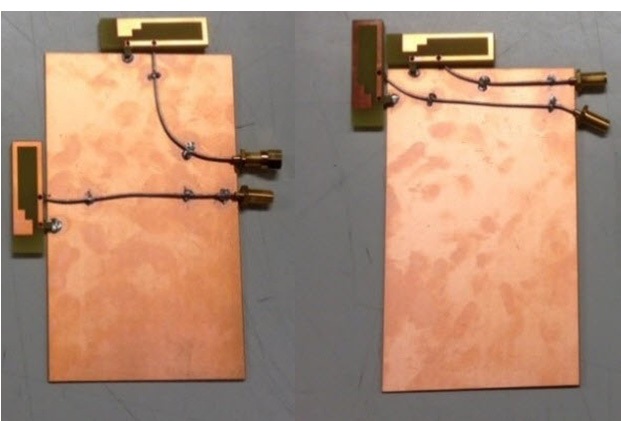
To validate the theory, an experiment is conducted using the Corner model and the Middle model as shown in Fig. 10. In the simulation, a MoM-based EM simulator called FEKO is used.
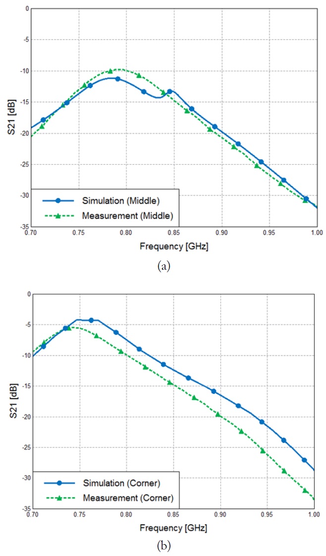
Fig. 11 shows the coupling,
Moreover, the current distributions of the Middle model are more orthogonal than those of the Corner model (Figs. 12 and 13).
Therefore, we are able to compare the coupling of the Middle model and the Corner model (–10 dB and –5 dB, respectively). We verify that the Middle model has a lower coupling tendency than the Corner model, thus validating the
In this paper, we proposed the usefulness of the
Two main approaches were used, namely, using the Booster and using a radiator. When using the Booster structure, which is electrically small whether it is attached or not, no significant change was observed. However, when using a radiator, which has an electrically large structure, a significant change in the ground plane’s CMA property was observed. Based on CMA, the Booster structure is more useful than a radiator in exciting a specific mode.
We also considered the coupling problem between dual radiators mounted on the same ground plane. Each radiator produces its own mode current. Therefore, we can compare the correlation to explain the coupling effect and validate this finding with other parameters (e.g., ECC and