Recently, the wireless power transfer (WPT) technology has become more important, and products related to single-input single-output (SISO) WPT systems have been globally commercialized with the example of wireless charging pads [1]. To expand the WPT market, regulatory issues regarding WPT commercialization and standardization are being finalized [2]. The WPT systems with multiple transmitters or multiple receivers have also been studied [3–5]. In [3], multiple-input single-output (MISO) WPT systems were investigated using closed-form solutions for the maximum WPT efficiencies. An analysis of the WPT efficiencies considering the multiple-output system was provided in [4]. Multiple-input multiple-output (MIMO) WPT systems including a repeater with a misalignment angle were examined in [5].
Still, there are many problems left in WPT systems, such as low efficiency, realization, stability, adaptability to mobility, EMI/EMC/EMF, and so on. In this paper, the WPT problem for general MIMO systems is formulated to achieve maximum efficiencies based on optimum loads. The maximum efficiencies of the systems can be obtained systematically for any number of transmitters and receivers. With this formulation, the optimum loads for maximum efficiencies can always be found at least numerically through a proper systematic optimization process. For some special cases such as SISO, SIMO, and MISO, closed-form expressions for the efficiencies and optimum loads for maximum efficiencies are derived and examined with various examples. The validity of circuit- and EM-simulated efficiencies are compared with the theoretical efficiencies.
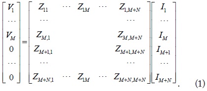
Fig. 1 shows a WPT system consisting of transmitters with a number of M and receivers with a number of N. They are assumed to be made of loops that have some inductances L. Each loop is loaded with a capacitor for resonance at a specific angular frequency ω0. Then, the Z matrix for the WPT system is given by
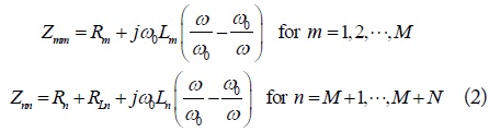
In (1), the elements in the column matrix [V] are the supplied voltages. The supplied voltages of the receiving loops are assumed to be zero. The diagonal and off-diagonal elements of the Z matrix as a function of angular frequency ω are expressed as
and
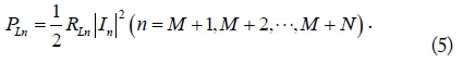
respectively. In (2), Rm (m = 1, 2, ⋯, M + N) is the loss resistance of each loop, and RLn (n = M + 1, M + 2, ⋯, M + N) is the load resistance of each receiver. In (3), kmn is the coupling coefficient [6].
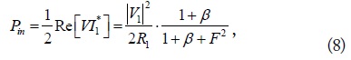
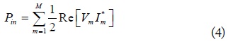
At the resonant angular frequency (ω0), the diagonal and offdiagonal elements in [Z] are shown to become purely resistive and purely imaginary, respectively. The current is determined by [I] = [Z]-1[V]. Then, the total input power and the received power at nth receiver are readily obtained by
and
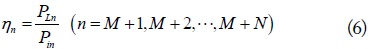
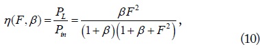
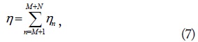
The WPT efficiencies for the nth receiver and the whole receivers are simply given by
and
respectively. Based on this formulation, the WPT efficiencies for any MIMO configurations with arbitrary loads RLn (n = M + 1, ⋯, M + N) can be evaluated. For design problems to maximize (6) or (7), the solutions for RLn (n = M + 1, ⋯, M + N) can be obtained at least numerically using Genetic Algorithm (evolutionary algorithm), which is a proper optimization algorithm. For some special cases of MIMO WPT systems such as SISO, SIMO, and MISO, we also try to analyze them analytically if possible.
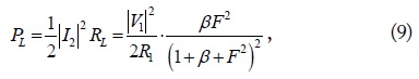
When the number of transmitting and receiving loops is 1 (M = N = 1, SISO), all solutions are already well- known but are repeated here for readers’ convenience. The transmitted power Pin, received power PL, and the WPT efficiency are given by [7]
and
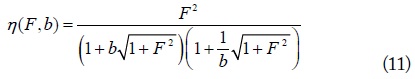
respectively, where the normalized load β (= RL/R2) and the figure of merit F (= kQ) are independent variables to determine the efficiencies. Q is the geometric mean of Q1 and Q2 and each is given by ω0L/R. It is known that (10) can also be expressed as

where b (= RL/RL,opt = β / βopt ) is the normalized load resistance referenced to the optimum RL,opt with which the maximum efficiency is achieved. βopt is the normalized optimum load resistance for maximum efficiency, given by [6,7]. When b = 1, the efficiency in (11) becomes maximum. When b is greater or less than 1, the two-loop WPT system becomes under-coupled or over-coupled, respectively, and the efficiencies decrease. It is interesting to observe that as F (= kQ) becomes smaller, RL,opt also becomes smaller. The condition of RL,opt = R2 when F = 0 (two loops placed far apart) reminds us of the condition of the maximum received power of an Rx antenna in the far field. It is also notable that even though the role of Tx and Rx loops are interchanged, the efficiency remains the same with a similar use of the optimum load.
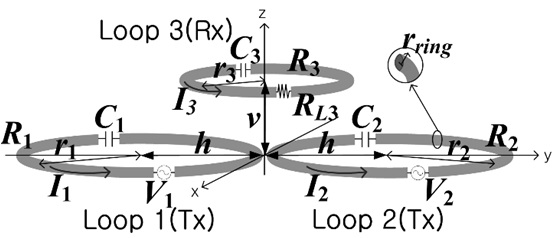
Fig. 2 shows a WPT system consisting of one transmitter and two receivers. The center positions of each loop are assumed to be at (0, 0, 0), (0, -h, v), and (0, h, v), respectively. We can analyze the system using a simple 3×3 Z matrix using (1)–(3).
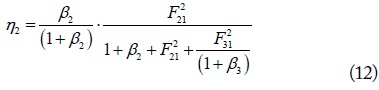
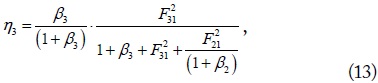
When the distance between the two receiving loops is large, the coupling coefficient k32 is negligibly small and can be assumed to be zero. For this case, the WPT efficiency of each loop can be expressed as
and
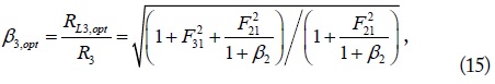
where Fn1 is the figure of merit defined by Qn is the quality factor given by ω0Ln/Rn, and βn is the normalized load resistance defined by RLn/Rn. The total WPT efficiency η is the sum of (12) and (13) as defined in (7). The normalized optimum load resistances β2,opt and β3,opt with which (12) and (13) are maximized can be shown to be given by
and
respectively. When β3→∞ (open) in (14), loop 3 becomes inactive (under-coupled limit), (normalized optimum load for the SISO WPT system). When β3→0 (short, over-coupled limit), The solution of RL2 and RL3 for the maximum η (= η2 + η3) may also be numerically determined with GA.
All the efficiencies and optimum loads evaluated and presented in this paper have been checked between the GA results based on (2)–(7) and circuit/EM-simulation results. The efficiencies and optimum loads have been found to be always in good agreement.
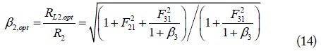
Fig. 3(a) and (b) show the maximum WPT efficiencies and the optimum load resistances for the case described in Fig. 2. The resonant frequency is 6.78 MHz, r1 = 15 cm, r2 = r3 = 5 cm, and rring = 0.2 cm. The Q-factors for the loops with r1 = 15 cm and r2 = r3 = 5 cm are about 730 and 560, respectively.
In Fig. 3(a), the efficiency η (= η2 + η3) are plotted as a function of h for v = 3 cm, 5 cm, and 7.5 cm. Besides, for the purpose of comparison, we have also plotted η2 when v = 3 cm without loop 3. It is shown that when h is smaller than roughly the radius of the Tx loop 1 (15 cm), η2 without loop 3 is greater than 90%, and it is almost the same as the total efficiency η (= η2 + η3) with both loop 2 and loop 3 symmetrically placed.
This means that when the Rx loops are properly placed in symmetry relative to the Tx loop, the nearly 100% efficiency can be shared by the receiving loops. When h is roughly between 17 cm and 20 cm, the efficiencies drastically drop to zero. These zero-efficiency phenomena occur at positions where the upward magnetic flux lines crossing a receiving loop change their directions and fall down into the loop again such that the net magnetic flux crossing the loop is zero. This corresponds to the zero-coupling coefficients (k).
Beyond the zero-efficiency (or the zero-coupling coefficient) positions, the net magnetic flux lines on the receiving loops go downward (the negative k changes only the direction of currents on the receiving loops), and the efficiencies are shown to increase to about 80% to 90% , but decrease again as h becomes large.
In Fig. 3(b), we show RL2,opt (= RL3,opt) as a function of v and h. When the distance between the Tx and Rx loops becomes large, RL,opt may become too small to be realized. This can be handled with a multi-turn Rx loop or an additional feeding loop or matching circuit [8–10] depending on the system requirements.
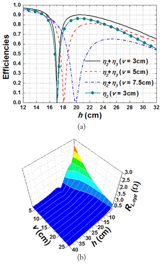
Fig. 4 shows the coupling coefficients k21, k31, and k32 depending on the distances v and h based on the same system configuration as described in Fig. 3. The coupling coefficients k’s were extracted based on [6]. These extracted coupling coefficients were checked to be the same as those obtained by [11]. As explained with Fig. 3(a), k21 and k31 (the coupling coefficients between the transmitting and receiving loops) are shown to be negative, zero, and positive depending on the loop 1 and loop 2 (or loop 3) positions. Due to the particular placements of loop 2 and loop 3 on a horizontal plane, k32 in Fig. 4(b) is always negative.
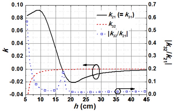
Fig. 5 shows the coupling coefficients k21 (= k31), k32, and |k32/k21| depending on the distance h with the fixed v of 3 cm based on the system configuration as described in Fig. 4. By evaluating |k32/k21| depending on the horizontal separation h, we can determine the condition where k32 may be ignored. We can see that since |k32/k21| is very small (less than 0.3) when h > 10 cm and v = 3 cm, the solutions in (12)-(15) are more accurate in this region.
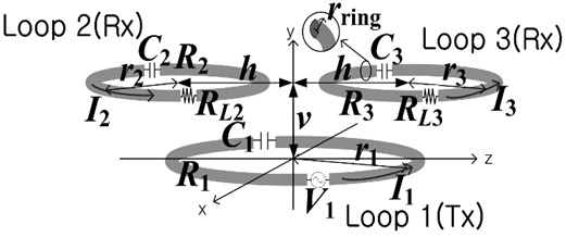
Fig. 6 shows a MISO configuration consisting two transmitters and one receiver. The center positions of each loop are (0, -h, 0), (0, h, 0), and (0, 0, v), respectively.
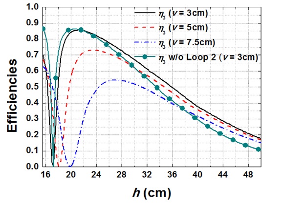
Fig. 7 shows the maximum WPT efficiencies for the system-described in Fig. 6. The resonant frequency is 6.78 MHz, V1 = V2, r1 = r2 = 15 cm, r3 = 5 cm, and rring = 0.2 cm. The Q-factors for the loops with r1 = r2 = 15 cm and r3 = 5 cm are about 730 and 560, respectively.
In Fig. 7, the maximum efficiency η3 are plotted as a function of h for v = 3 cm, 5 cm, and 7.5 cm. Besides, for the purpose of comparison, we have also plotted η3 without loop 2 when v = 3 cm. It is shown that when h is about 16 cm, η3 without loop 2 is approximately 90%, but η3 with loop 2 is somewhat less than 90%. When h is roughly between 17 cm and 20 cm, the efficiencies drastically drop to zero. Beyond the zero-efficiency (or the zero-coupling coefficient) positions, the efficiencies are shown to increase to about 55% to 85%, but decrease again as h becomes large.
Fig. 8 shows the coupling coefficients k21, k31, and k32 depending on the distances v and h under the same conditions as described in Fig. 7.
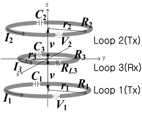
Fig. 9 shows a MISO system (M = 2, N = 1) with two vertically placed transmitters. The center positions of each loop are (0, 0, -v), (0, 0, v), and (0, 0, 0), respectively.
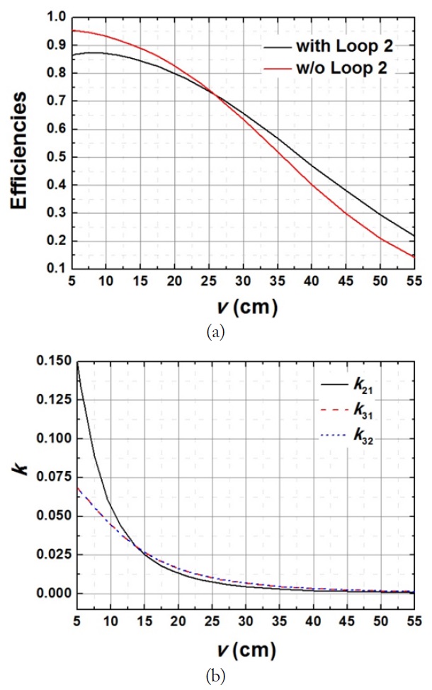
Fig. 10(a) and (b) show the WPT efficiency η3 and coupling coefficients for the case described in Fig. 9. The resonant frequency is 6.78 MHz, V1 = V2, r1 = r2 = 15 cm, r3 = 5 cm, and rring = 0.2 cm. The Q-factors for the loops with r1 = r2 = 15 cm and r3 = 5 cm are about 730 and 560, respectively. In Fig. 10(a), the maximum efficiencies η3 with and without loop 2 are plotted as a function of v. For the purpose of comparison, we have also plotted η3 without loop 2.
When v is smaller than 26 cm, η3 without loop 2 is somewhat greater than η3 with loop 2. When v is larger than 26 cm, the opposite is true. As v increases, the benefit of using two Tx loops is shown to be more significant.
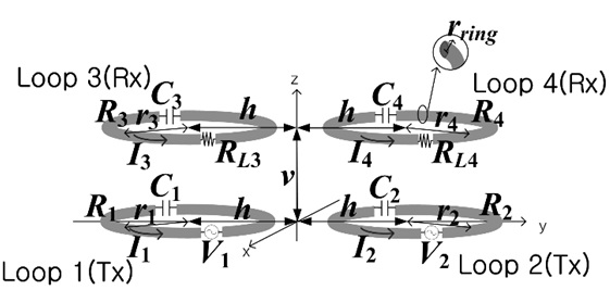
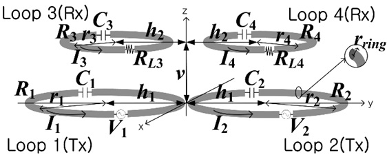
Fig. 11 shows a MIMO system (M = 2, N = 2). Performances of this system can also be analyzed using the formulation (1)–(7).
[Fig. 11.] A MIMO system (M = 2, N = 2) with two horizontally placed transmitters and receivers. Each loop is located at (0, -h1, 0), (0, h1, 0), (0, -h2, v), and (0, h2, v).
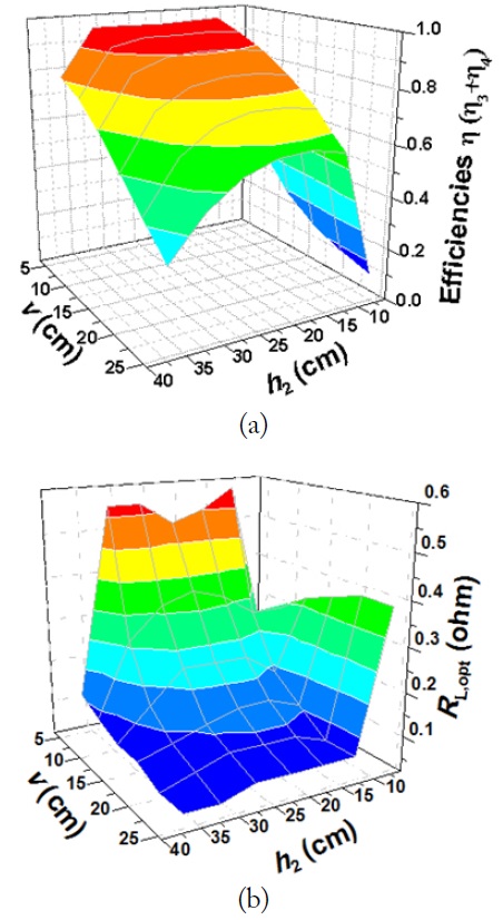
Fig. 12(a) and (b) show the WPT efficiencies and the optimum load resistances for the case described in Fig. 10. The resonant frequency is 6.78 MHz, V1 = V2, r1 = r2 = 15 cm, r3 = r4 = 5 cm, rring = 0.2 cm, and h1 = 20 cm. The Q-factors for the loops with r1 = r2 = 15 cm and r3 = r4 = 5 cm are about 730 and 560, respectively.
In Fig. 12(a), η (= η3 + η4) are plotted as a function of v and h2. It is shown that when 5 cm ≤ v ≤ 15 cm and 10 cm ≤ h2 ≤ 30 cm, η (= η3 + η4) is well above 90%. In Fig. 12(b), RL,opt is shown to be about 0.5 Ω when v is 5 cm and 30 cm ≤ h2 ≤ 35 cm.
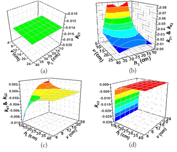
Fig. 13 shows the coupling coefficients k21, k31, k32, k41, k42, and k43 depending on the distances v and h2 under the same conditions as described in Fig. 12. In Fig. 13(a), k21 (the coupling coefficients between the transmitting loops) is about -0.0014. In Fig. 13(c), k41 and k32 (the coupling coefficients between the transmitting and receiving loops that are located diagonally) are shown to be negative, zero, and positive, depending on the loop positions.
[Fig. 13.] Coupling coefficients at 6.78 MHz with V1 = V2 as function of v and h2 (r1 = r2 = 15 cm, r3 = r4 = 5 cm, rring = 0.2 cm, h1 = 20 cm, Q1 = Q2 = 730, Q3 = Q4 = 560). (a) k21, (b) k31, k32, (c) k41, k42, and (d) k43.
Since the MIMO WPT systems are considered to be a natural extension of the SISO system, the overall WPT system efficiencies have been found to be well above 90% when the distances between the TX and Rx loops are roughly less than the radius of the Tx loops.
Fig. 14 shows a MIMO system (M = 2, N = 2). Performances of this system can also be analyzed using (1)–(7).
[Fig. 14.] A MIMO system (M = 2, N = 2) with two horizontally placed transmitters and receivers. Each loop is located at (0, -h, 0), (0, h, 0), (0, -h, v), and (0, h, v).
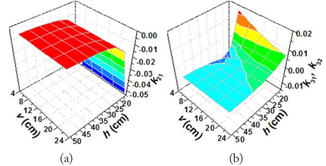
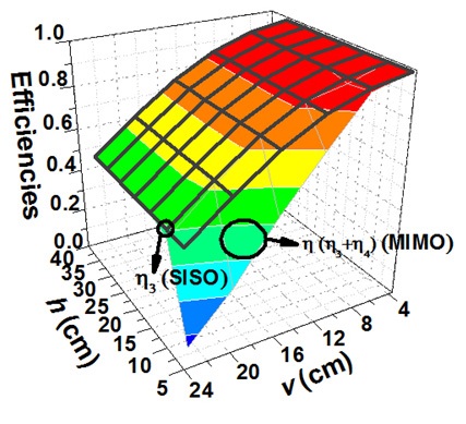
Fig. 15 shows the WPT efficiencies for the case described with all loops (MIMO) or without loop 2 and loop 4 (SISO) in Fig. 14. The resonant frequency is 6.78 MHz, V1 = V2, r1 = r2 = r3 = r4 = 5 cm, rring = 0.2 cm. The Q-factors for the loops with r1 = r2 = r3 = r4 = 5 cm are about 560.
In Fig. 15, η (= η3 + η4) (MIMO) and η3 (SISO) are plotted as a function of v and h. It is shown that when 4 cm ≤ v ≤ 8 cm, η (= η3 + η4) (MIMO) and η3 (SISO) are well above 90%. It is shown that η (= η3 + η4) (MIMO) becomes smaller as the vertical separation v becomes larger. η (= η3 + η4) (MIMO) is about 0.1–0.6 when 5 cm ≤ h ≤ 10 cm and 14 cm ≤ v ≤ 24 cm. It becomes smaller than η3 (SISO) since η (= η3 + η4) (MIMO) is affected by the coupling of the four loops. This implies that it is more effective to use a SISO system when 5 cm ≤ h ≤ 10 cm than to use a MIMO system.
Although the EM simulation results have been analyzed and discussed up to M = 2 and N = 2 systems, MIMO WPT systems with more Tx and Rx loops are expected to have similar performance behaviors.
In particular, for the WPT system with M = 1 and arbitrary N, the efficiencies of the Rx loops have been found to be shared among them, and the total efficiency can be engineered up to 1 depending on the system configurations.
We formulated the MIMO WPT systems in terms of transfer efficiencies for each receiver and the whole receivers. The optimum loads of the receivers for the maximum WPT efficiencies have been shown to be found at least numerically based on the formulation. For some typical special cases of SISO, MISO, and SIMO system have been analyzed using circuit- and EM-simulations together with the derived closed-form solutions. In particular, the SIMO system has been shown to be effective in that the near 100% efficiency can be shared by the receiving loops. The derived closed-form solutions have been demonstrated to give us plentiful physical insight for the systems. The results of this paper may be useful to construct WPT systems for Internet of Things requiring sensors with energy autonomy without batteries.