The recent financial crisis has highlighted the interconnectedness between macroeconomic and financial stability. In particular, the housing sector is pivotal in understanding the recent financial crisis. When the house market collapsed with subprime mortgage, microprudential policies that prevent the risk faced by each company could not prevent the crisis from spreading across the financial and housing sectors in the real econ-omy. The traditional monetary policy is not sufficient to avoid the crisis and gain a robust recovery. Since the outbreak of the Great Recession, many economists have realized that the existing set of monetary policies aimed at price stability and the microprudential regulations targeted at the financial soundness of individual banking institutions are insufficient in stabilizing the economy from financial shocks.
The set of macroprudential policy tools are now being discussed and introduced in advanced economies. Some governments have already implemented macroprudential tools to promote the stability of the financial system and to minimize the transmission of financial shocks to the entire economy. For example, in the Korean economy, a household's relatively high leverage ratio is more vulnerable to shocks (
Given that macroprudential policy inevitably interacts with monetary policy, the question of whether or not and how monetary and macroprudential policy makers should respond to financial variables warrants a close look. Some examples of macroprudential policy tools are capitalbased tools (
Abel (1990) and Campbell and Cochrane (1999) postulate that envy is one of the most important elements in human behavior, particularly in explaining preferences related to the rising household leverages in many industrial countries. In the present study, we incorporate the idea of “catching up with the Joneses” along the lines of Ljungqvist and Uhlig (2000) and Campbell and Cochrane (1999) into a canonical sticky price model. Given that the agents are determined to catch up with the Joneses without considering the effects of such behavior on aggregate demand, they unconsciously overheat the economy in expansionary phases and cool it down excessively in contractionary phases. This kind of external habit formation, which generates unnecessary fluctuations in the economy over the business cycle, calls for a more active government stabili-zation policy.
In the present study, we establish a simple sticky price model that features the housing market to discuss how monetary and macroprudential authority should react to exogenous shocks. The benchmark model is similar to that of Iacoviello (2005) with two-types of households: borrowers and savers. Impatient borrowers face the collateral constraint linked to the expected market value of their houses and labor income, whereas patient savers smoothen their consumption profile with their financial assets. We then evaluate the implications of time-varying versus time-invariant macroprudential policies, such as the LTV and DTI tools, and their interaction with the monetary policy related to financial stability and business cycles. We specifically address how the macroprudential and monetary authority react to exogenous shocks. For this purpose, we introduce into the model two kinds of simple and implementable macroprudential rules as the Taylor-type interest rate rule. The macroprudential authority responds to either the credit growth or house price growth to avoid episodes of excessive credit growth in the spirit of the Basel III regulation.
The main findings of this study can be summarized as follows: First, time-varying macroprudential policy is more effective in stabilizing household debt than time-invariant macroprudential policy, whether or not the macroprudential authority accounts for a borrower's labor income, in addition to the LTV in the macroprudential policy.
Second, macroprudential policy based on the pure LTV ratio is better in moderating household debt to house demand shock than macroprudential policy that accounts for both the borrower's labor income and market value of the house.
Finally, macroprudential policy that accounts for both the borrower's labor income and the market value of the house is better in moderating household debt to productivity shock than the macroprudential policy based on the pure LTV ratio.
The remainder of this paper is organized as follows: Section II presents an experience of the Korean economy. Section III presents a canonical sticky price model augmented with collateral constraints. Section IV discusses the simple, implementable, and optimal Taylor rule and macroprudential policy and compares the properties of monetary and macroprudential policy rules. Section V ends with a conclusion.
1The LTV limits are available in 16 member states of the EU.
II. An Experience of the Korean Economy
Korea is one of the few countries that are in the forefront of macroprudential policy implementation. Some of the stylized facts of the Korean economy are illustrated in this section.
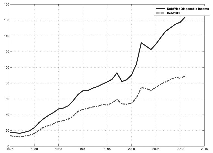
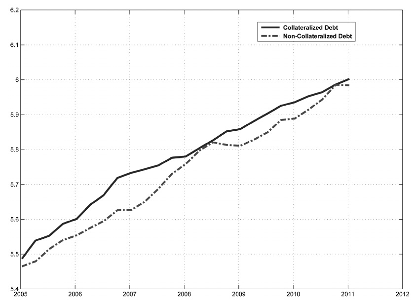
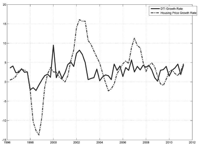
Figure 1 shows the household debt to disposable income ratio in Korea. The debt to income ratio increases about 5-10% per year, except during the credit card crisis in 2003. Figure 2 shows that the household's collateralized debt increased to 20% at the beginning of 2000. The high ratio of collateralized debt indicates that households rely on banks to finance Chonse or mortgage loans.
Korea implemented its macroprudential tool in 2002 to address the rapid increase in house prices with LTVs. To moderate the house market fluctuation, the Korean government also introduced DTIl in 2005, along with tax incentives/disincentives and direct/indirect support to the construction sector. Figure 3 shows the annual growth rate of the Korean house price since 2000. Despite the Korean government's strategy of tightening the LTV across banking and non-banking financial institutions, the monetary policy has been relatively loosened. The mixed result of a relatively high growth rate and reduced variations in house prices may reflect this policy mix. The exploration of the consequences of lax monetary policy and tight macroprudential policy in terms of price and financial stability is interesting.
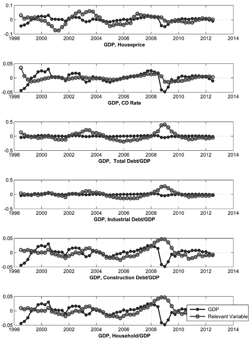
Figure 4 shows the band pass filter series of selected variables, such as GDP, real housing price, and various debt ratios relative to GDP. Features of business cycles in terms of cross autocorrelations are useful in examining the features of debt variables. Table 1 shows various moments of the selected variables calculated from the estimated spectral density matrix with only the business cycle (6-32 quarter) frequencies of Korea. The nominal interest rate is an inverted leading indicator over business cycles (corr(
[TABLE 1] MOMENTS OF DATA (1998:III-2012:III)
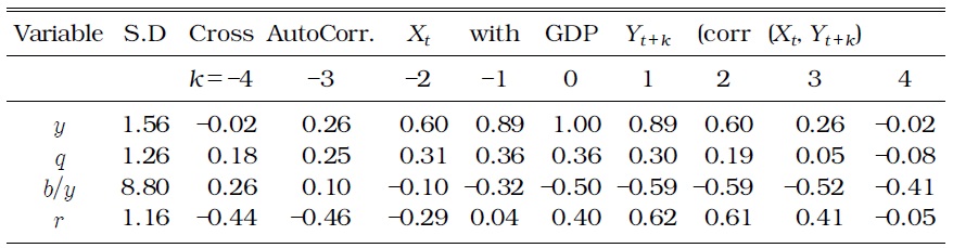
MOMENTS OF DATA (1998:III-2012:III)
We set up a model with the housing sector based on that of Iacoviello (2005). The economy consists of savers, borrowers, final goods firms, and the government. Each household supplies labor and consumes both consumption goods and housing services.
Savers maximize their expected life-time utility by choosing consumption, housing, and working hours:
Abel (1990, 1999) and Smets and Wouters (2007) specify a simple recursive preference, in which a representative household derives utility from the level of consumption relative to a time-varying subsistence or habit level. We particularly assume that the utility function of a representative household takes the form

where
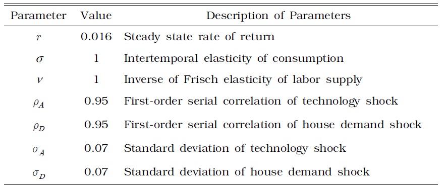
[TABLE 2] CALIBRATED PARAMETERS

CALIBRATED PARAMETERS
The saver faces the following budget constraint:
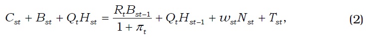
where
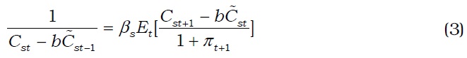
The first-order conditions are given by


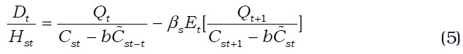
Equation (3) is a standard Euler equation, which states that a saver's consumption depends on the real interest rate. Equations (4) and (5) are a standard condition for labor supply and an intertemporal condition for housing service, respectively.
Borrowers maximize the utility function

where
The borrower faces a collateral constraint in addition to the budget constraint


where
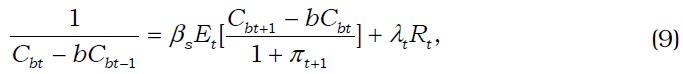
The first-order conditions are given by


where
Next, suppose that the government implements a more general macroprudential policy by combining the DTI constraints and collateral constraints, as in Gelain

where

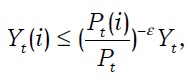
Differentiated goods and monopolistic competition are introduced, as in Dixit and Stiglitz (1977). A continuum of firms that produce differentiated goods exists, and each firm that is indexed by

where At is the productivity shock that follows an AR(1) process as log
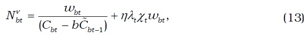
Equation (15) implies that the labor efforts of the savers and borrowers are not perfect substitutes, as in Iacoviello (2005). Firm i's demand for labor is determined by its cost minimization as follows:
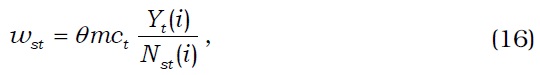
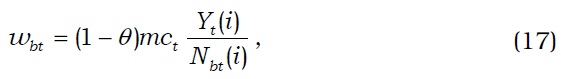
where
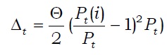
Much research has been conducted on the price decision rules in monopolistically competitive product markets. In this subsection, a Rotemberg-type of price setting is considered. To introduce the nominal price rigidities in the model, suppose that the representative firm

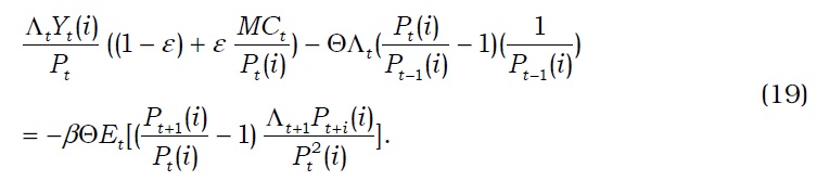
The monopolistically competitive firms in the goods markets set their own prices by maximizing the present discounted value of profits. The firm's maximization problem is written as follows:

subject to

where Λ
The newly determined prices at time
We consider a Taylor rule, which corresponds to the inflation and output gap:
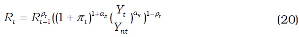
where
We introduce macroprudential policy in terms of the regulations of LTV ratios as a way of maintaining credit market stability. We assume that a countercyclical Taylor-type macroprudential policy exists for LTV ratios; thus, it responds to the credit market status in the spirit of the Basel III regulations.
Two kinds of time-varying macroprudential policy are considered. First, the LTV ratio responds negatively to credit growth as shown by
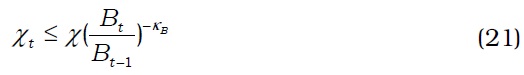
where
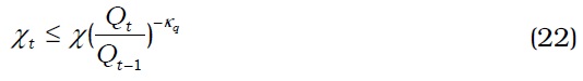
Second, the LTV ratio is assumed to negatively respond to the housing price growth.

where
a) Equilibrium
A symmetric equilibrium implies that all firms set the same price and choose the same demand for labor:
In such equilibrium, Equation (19) is simplified into

The clearing of the goods market requires that
The total supply of housing is fixed and is normalized to unity:

2See Iacoviello (2005), who finds no stabilization effect for a generalized Taylor rule.
All the parameter values used in this study are listed in Table 1. The discount factor for savers
The benchmark model of this study takes the value of the intertemporal elasticity of substitution and labor supply elasticity as equal to one, that is,
>
B. Optimized Monetary and Macroprudential Rules
To characterize an optimal, simple, and implementable monetary and macroprudential policy, social welfare must be defined. Suppose that the government assigns the weight

The values
In the optimized rules, the policy parameters
The weight assigned to savers versus borrowers is very important in evaluating the optimized interest rate rule and macroprudential rule. Macroprudential policy improves financial stability by dampening the borrower's debt and makes the borrower's welfare better off (worse off), while it makes the saver's welfare worse off (better off) in many cases. A trade-off occurs between savers and borrowers in terms of welfare as the LTV ratio changes. For example, Campbell and Hercowitz (2009) show that a higher LTV ratio harms borrowers, whereas savers benefit from the increase. A higher LTV ratio implies that borrowers accept higher consumption profiles, given that borrowing constraints are always binding. However, higher consumption levels imply a higher interest rate, which increases both borrower's debt burden and saver's returns on savings. In this study, the weight
>
C. Macroprudential Policy with LTV Only
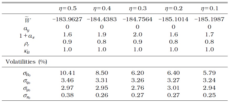
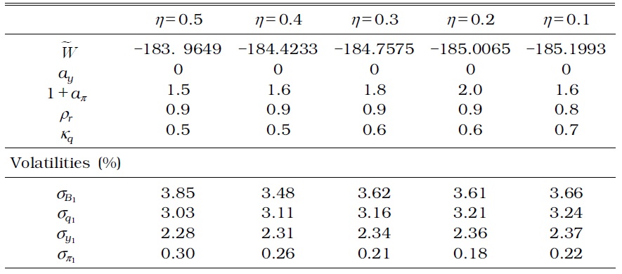
Consider the macroprudential policy augmented with Equation (21). Table 3 presents the optimized parameter values, volatilities of selected variables, and the corresponding welfare when the monetary authority implements a time-invariant macroprudential policy, whereas Table 4 presents the results when the monetary authority implements a timevarying macroprudential policy.
OPTIMAL MONETARY AND MACROPRUDENTIAL POLICY PARAMETERS IN A MODEL WITH ONLY A TIME-INVARIANT LTV (η=0)

OPTIMAL MONETARY AND MACROPRUDENTIAL POLICY PARAMETERS IN A MODEL WITH ONLY A TIME-VARYING LTV (η=0)
No difference exists between a time-invariant and time-varying macroprudential policy, except for household debt volatility. The time-varying macroprudential policy successfully reduces household debt fluctuations, whether or not the authority reacts to the credit growth rate or house price growth rate.
a) Dynamic Effects of Productivity Shocks
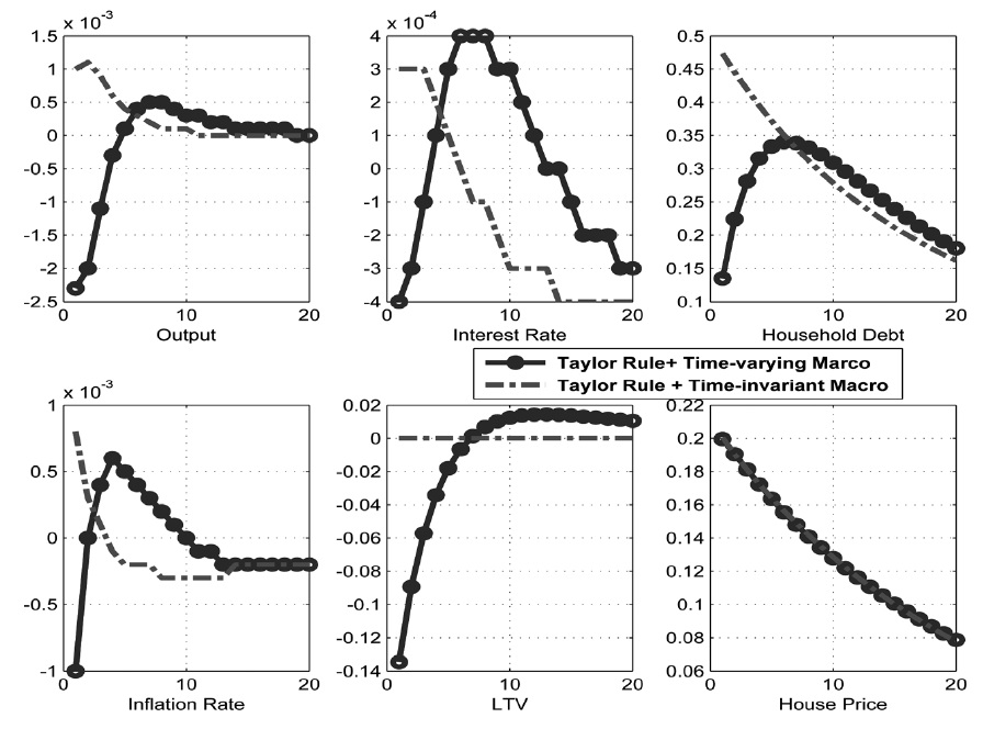
Consider the effect of productivity shock on the economy without habit persistence in consumption. The circles in Figure 5 represent the impulse response function to the positive productivity shock when the monetary authority implements an optimized Taylor rule, and the macroprudential authority implements an optimized time-varying macroprudential policy. The long-dashed lines represent the response of the corresponding vari ables from the steady state when the monetary authority implements a Taylor rule, and the macroprudential authority implements a time-invariant macroprudential policy. A positive productivity shock results in an increase in output and a decrease in interest rate.
Given the expansion in the economy, the demands for house and loans increase and lead an increase of house price. Without a time-varying macroprudential policy that reacts to credit growth rate, the LTV ratio remains constant, and household debt instantaneously increases. However, household debt does not increase as much as it does in a timeinvariant macroprudential policy, when a time-varying macroprudential policy is in place because the LTV ratio decreases.
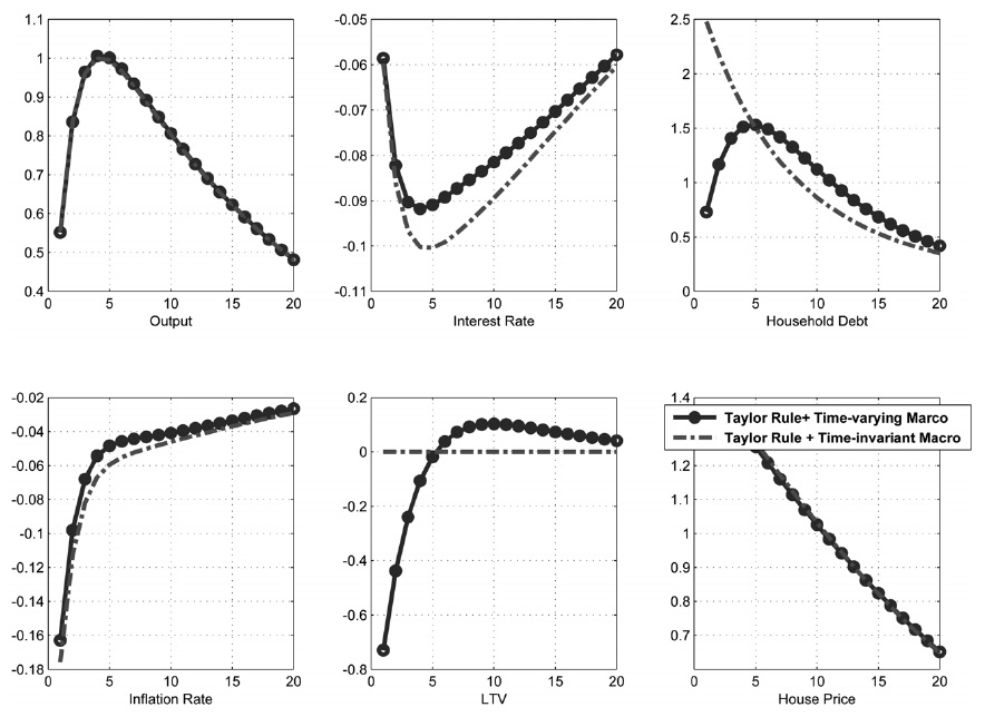
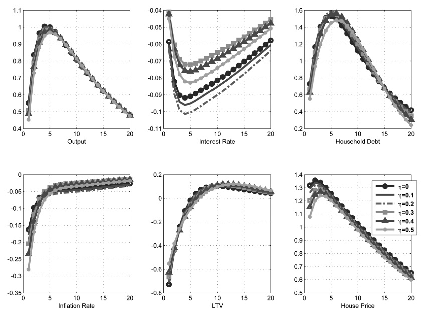
Consider the effect of productivity shock on the economy with external habit persistence on consumption. As in Figure 6, the output, household debt, and house prices respond more strongly to productivity shocks in an economy with external habit than in an economy without external habit, because households with an external habit are determined to catch up with the Joneses without considering the effects of such behavior on aggregate demand. They unconsciously overheat the economy in expan sionary phases and cool it down excessively in contractionary phases, thereby generating unnecessary fluctuations in the economy over the business cycle. The comparison of circles and long-dashed lines in Figure 6 shows that the time-varying macroprudential policy is more effective in moderating the increase in household debt than the time-invariant macroprudential policy.
b) Dynamic Effects of House Demand Shocks
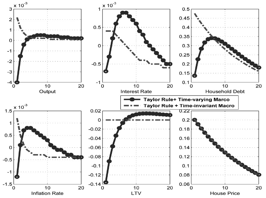
Consider the effect of housing demand shock on an economy without any habit. The circles in Figure 7 display the response of the variables when the monetary and macroprudential authorities implement an optimized Taylor rule and time-varying macroprudential rule, whereas the long-dashed lines represent the response of the corresponding variables when the said authorities implement an optimized Taylor rule and timeinvariant macroprudential rule. Given the increase in house prices, the loan increases. Borrowers can borrow more from their housing collateral, which is worth more. However, when the macroprudential authority cooperates with the monetary authority with time-varying macroprudential policy to moderate the boom in housing sector, the LTV ratio decreases, and the household debt does not increase as much as that with a time-invariant macroprudential policy.
Next, consider the effect of housing demand shock on consumption, when households have an external habit. The compression of circles and long-dashed lines in Figure 8 shows that time-varying macroprudential policy is more effective in moderating the increase in household debt than the time-invariant macroprudential policy.
c) Generalized Macroprudential Policy
In this subsection, we consider the generalized macroprudential policy that incorporates DTI and LTV to enhance the financial stability given by Equation (6). Under this specification, the macroprudential authority can change the value of
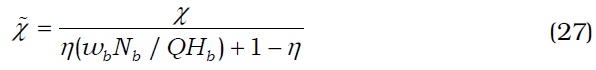
For example, =0.8802 when
Tables 5-8 present the optimized parameter values, volatilities of selected variables, and the corresponding welfare.

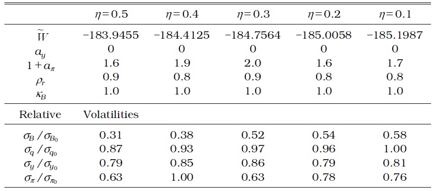
OPTIMIZED MONETARY AND MACROPRUDENTIAL POLICY PARAMETERS IN A MODEL WITH TIME-INVARIANT LTV AND DTI
OPTIMIZED MONETARY AND MACROPRUDENTIAL POLICY PARAMETERS IN A MODEL WITH TIME-VARYING LTV AND DTI

OPTIMAL MONETARY AND MACROPRUDENTIAL POLICY PARAMETERS IN A MODEL WITH TIME-INVARIANT LTV AND DTI
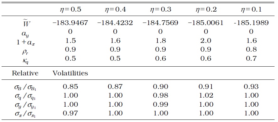
OPTIMAL MONETARY AND MACROPRUDENTIAL POLICY PARAMETERS IN A MODEL WITH TIME-VARYING LTV AND DTI
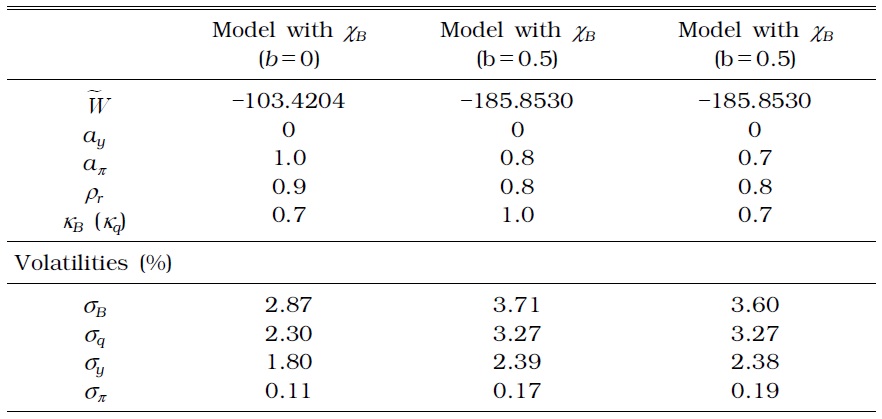
First, household debt fluctuation increases when the macroprudential authority considers a time-invariant DTI ratio, in addition to a timeinvariant LTV ratio, in collateral constraints. Although the LTV ratio in a generalized macroprudential policy as specified by Equation (12) moves endogenously to exogenous shocks, it is not enough to curb the excessive fluctuation of household debt. Tables 5 and 7 show that the time-invariant DTI fails to moderate household debt fluctuations with a borrower's labor income fluctuation over business cycles.
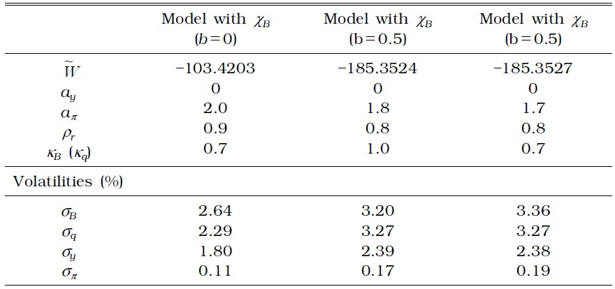
Second, a time-varying macroprudential policy results in a large stabilization effect on household debt more than a time-invariant macroprudential policy as shown in Tables 6 and 8. The standard deviation of all the other relevant variables also decreases, regardless of the weight (
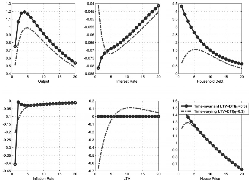
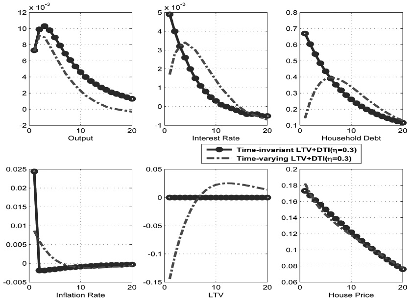
d) Dynamic Effects of Productivity Shocks
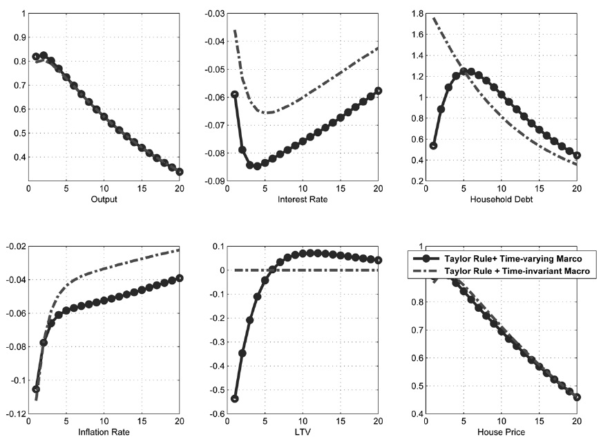
First, consider the effect of productivity shock on the economy. The circles in Figure 9 represent the impulse response function to the positive productivity shock when the monetary authority implements an optimized Taylor rule and the macroprudential authority implements optimized time-varying macroprudential policy. The long-dashed lines represent the response of the corresponding variables from the steady state when the monetary authority implements a Taylor rule and the macroprudential authority implements a time-invariant macroprudential policy.
Given the expansion in the economy, the demands for house and house price increase. As the increase in the borrower's labor income loosens the collateral constraints, household debt is given more room to increase even if a time-invariant macroprudential policy that reacts to credit growth or house price growth is in place. However, the increase in the household debt dampens when the macroprudential authority reacts to its generalized LTV ratio to the credit growth or house price growth. Output expansion also tends to be muted with the implementation of a time-varying macroprudential policy.
The comparison of the circles and long-dashed lines in Figure 9 shows that a time-varying macroprudential policy is more effective in moderating the increase in household debt than a time-invariant macroprudential policy.
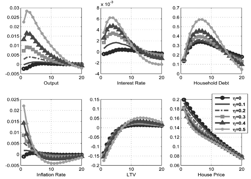
Figure 10 shows the dynamic effects of productivity shock on the economy when the weight to the borrowers (
e) Dynamic Effects of House Demand Shocks
Consider the effect of housing demand shock in the economy. The circles in Figure 11 display the response of the variables when the monetary and macroprudential authorities implement an optimized Taylor rule and time-varying macroprudential rule, whereas the long-dashed lines represent the response of the corresponding variables when the monetary and macroprudential authorities implement an optimized Taylor rule and time-invariant macroprudential rule. Given the increase in house prices, the loan increases. Borrowers can borrow more from their housing collateral, which is worth more. Moreover, the induced expansion of the real economy increases a borrower's labor income, giving more room for household debt to increase. However, when the macroprudential authority cooperates with the monetary authority in employing a timevarying macroprudential policy to moderate the boom in the housing sector, the LTV ratio decreases, and household debt does not increase as much as it does in a time-invariant macroprudential policy.
Figure 12 shows the dynamic effects of house price shock on the economy when the weight of the borrowers (
3According to the Bank of Korea (2014), the net asset to GDP ratio equals 7.7, and the housing asset to GDP ratio equals 2.2. 4The rule should satisfy two requirements, the interest-rate rule and the macroprudential policy, both of which are functions of a small number of easily observable macroeconomic variables, which must deliver a unique rational expectation and induce nonnegative equilibrium dynamics for the nominal interest rate.
In this study, we develop a simple sticky price model that features the housing market and discuss how monetary and macroprudential authority should react to exogenous shocks. The benchmark model is similar to that of Iacoviello (2005) with two types of households. We find that a time-varying macroprudential policy is more effective in stabilizing household debt than a time-invariant macroprudential policy, whether or not the macroprudential authority considers the borrower's labor income, in addition to the LTV ratio, in macroprudential policy. Moreover, a macroprudential policy based on the pure LTV ratio is better in moderating household debt to the house demand shock than a macroprudential policy that accounts for both the borrower's labor income and the market value of the house.
As an extension, a rigorous optimal monetary and macroprudential policy analysis is needed in a fully articulated model augmented with commercial banks.