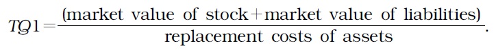
Firm value (hereafter FV) calibrates the efficiency of signaling a firm’s performance in the market, forecasts expected yields of investments, and assesses the realized efficiency of investments. Accordingly, scholars have improved the methodological precision in their estimates of FV. Currently, Tobin’s Q ratio (aka Tobin’s Q) (1969) is the most widely adopted measurement. This ratio constructs FV by using the ratio of market values of liabilities and stock to replacement costs of assets. The market value of a firm’s assets is obtained from the sum of the market values of stock and liabilities. Replacement costs represent the amount it would cost to replace an asset at its current price.
However, calculating Tobin’s Q accurately is not easy. The market values of stock and liabilities are difficult to estimate. Estimating replacement costs also requires consideration of various factors related to different types of assets, which complicates the computation. Therefore, many researchers tend to use book values rather than market values of liabilities and assets.
In several empirical studies, Tobin’s Q has been adopted as a key independent or dependent variable (Morck
Our estimation method follows Lindenberg and Ross (1981) and Hoshi and Kashyap (1990), who further developed the methodology of Tobin (1969). We compare existing methods and the differences in estimation results. We also make several important improvements, such as in the estimation of values of preferred stocks and replacement costs of assets. We estimate the values of preferred stocks following Lindenberg and Ross (1981) and Summers (1981), and divide average dividends by average dividend ratio. This method is better than others because prices of preferred stocks are not easily available due to less frequent transactions.
Improvement in the estimation of the replacement costs of assets hinges on the method of calculating depreciation rates. Hong
With this new estimation approach, we use the data of the Korea Information Service (KIS) Value, which is typically used in empirical papers on Korean firms. Therefore, we have the estimated values of Tobin’s Q for each listed firm from 1980 to 2005. The value of Korean firms changes during the time when year and industry effects are considered. However, we find that Tobin’s Q remains below one on average during most of the period. Before 1997, the value of stand-alone firms is significantly greater than that of business groups. After 1997, the situation is reversed. In addition, our estimation of the investment function shows that, depending upon the estimation approach, the statistical significance of the coefficient of the Tobin’s Q variable can vary, which indicates an imperative need to adopt more accurate values of Tobin’s Q.
In section II, we review and compare the existing approaches. We illustrate several concepts used to estimate the FV of listed firms in Korea and summarize the methodological issues for FV estimation. In section III, we provide the results of the FV estimates using different approaches and discuss their implications. In section IV, we estimate the investment function using the different methods of Tobin’s Q calculation to compare them. Finally in section V, we conclude this study.
II. Methodological Issues and Data
>
A. Defining Several Proxies and Variants of Tobin’s Q
As discussed above, people tend to use the

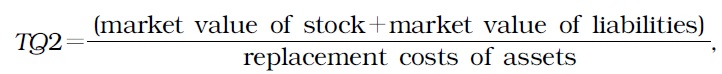
Then, a first improvement (or
However, both

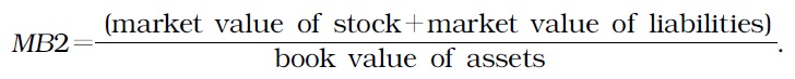
In our terminology,

where market value of stocks=①+②,
①=(year-end price of common stocks×number of outstanding common stocks)
②=(dividend of the preferred stocks÷dividend ratio of the preferred stocks)×number of outstanding preferred stocks
>
B. Methods to Estimate the Market Value of Stocks
In estimating the market value of stocks, common stocks are included and preferred stocks are only sometimes considered. The price of preferred stocks is unclear because of non-tradability or very low trading volume. Accordingly, Lindenberg and Ross (1981) and Summers (1981) obtain the price by dividing the dividends of preferred stocks by the S&P average dividend ratio. Therefore, we also divide the dividends of preferred stocks by the average dividend ratio of preferred stocks to calculate the price. Next, we multiply the number of both types of shares (common and preferred) by the matching prices. This process is how
>
C. Methods to Estimate the Market Value of Liabilities
We first consider the book value of liabilities from the total liabilities in the balance sheet. Then, the market value of liabilities can be calculated as the sum of (a), (b), (c), (d), and (e), which we explain below. The values of liabilities in the balance sheet or income statement are the book values at issuance, and thus they do not reflect time-varying factors, such as interest rate or price, which potentially affect the value of liabilities. Therefore, we categorize liabilities into non-interest-and interestbearing debts. As the book values of non-interest-bearing debts are equivalent to their market values, we can use the book values directly and calculate the market values as follows:
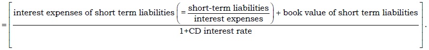
Second, given that interest-bearing debts must have different book values and market values, we obtain the market value of this type of debt by deriving the present values of interest payments and the principal, and then finding their sum. A typical financial statement (
Market value of short-term liabilities (b)

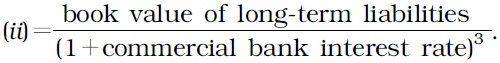
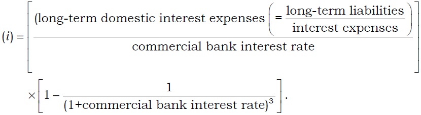
Long-term domestic liabilities (c)=long-term borrowings
Market value of long-term domestic liabilities (c)=(

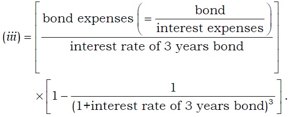
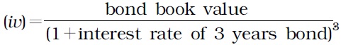
Bonds (d):
Market value of bond (d)=(


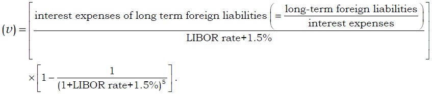
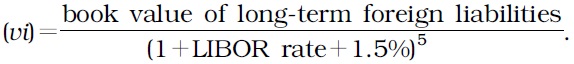
Long-term foreign liabilities (e)=long-term borrowings in foreign currency+overseas loans.
Market value of long-term foreign liabilities (e)=(
>
D. Methods to Estimate the Replacement Costs of Assets
This study calculates the replacement costs for Tobin’s Q as the sum of the replacement costs for quick assets, investment assets, inventory assets, intangible assets, and tangible assets. We use the current book value for quick assets and intangible assets, as their book values and replacement costs are considered equivalent, so we use the current data provided by the KIS Value. Valuation of investment assets varies depending on the time of evaluation of securities. Our study takes those reported in the KIS Value. Then, we follow Kim
Method A (
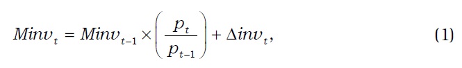
If the change in the value of inventory assets is greater than or equal to zero, we use Equation (1) as follows:

where
Δ
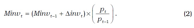
If the change in the value of inventory assets is less than zero, that is,
Δ

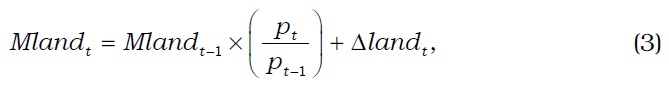
Second, the replacement costs of tangible assets are obtained from Equation (3) or (4) for land and from Equation (5) for other assets. If the change in the value of land is non-negative, we use Equation (3).

where
Δ
Δ
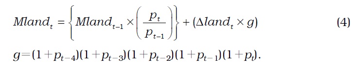
If the change in the value of land is less than zero, that is, Δ

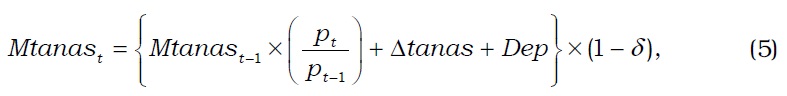
Third, for seven types of tangible assets other than land, the replacement costs are obtained as follows:

where
Δ
Method B (
where
We further discuss the two methods as follows. First, in response to the report of Kim
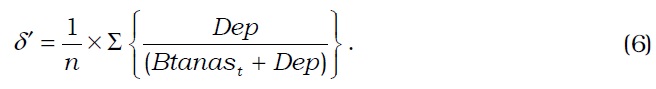
We use the economic depreciation rates for tangible assets in method A, as estimated by Hyun and Pyo (1997). However, their economic depreciation rates are derived from the estimation of capital stocks in the 1980s. As this study examines the period between 1980 and 2005, the application of the economic depreciation rates in the 1980s to a later period is inappropriate. Moreover, we do not recommend using a single economic depreciation rate (although the rate is categorized by type of asset) for all firms without allowing for across-firm differences. To overcome this problem, method B uses the annual average depreciation rates, as suggested by Kim
A problem with this approach is that negative depreciation rates can result when a smaller increase in accumulated depreciation (the Dep variable in Equation (6)) exists in the current year than in the previous year. Negative depreciation rates were actually obtained from many firms for many years before the crisis in 1997. Although divestiture (selling off assets on a large scale) provides a possible explanation, a question persists on whether Korean public firms were indeed selling off assets even before the Asian crisis in 1997. Although unused assets were undoubtedly disposed of after the crisis, Korean firms before the crisis had certainly overinvested. Kang and Shin (2004) argue that negative values may result because an accurate value of the depreciation rate for tangible assets cannot be known for each year. To remove negative values in the depreciation rates, Kang and Shin (2004) simply drop the years with smaller accumulated depreciation than the preceding year. This step is likely to result in the dropping of too many years and thus possibly lead to some bias in the process of obtaining the depreciation rate. Our alternative solution in method B is to use the amount of accumulated depreciation itself rather than the change in the amount. This way, we can avoid the negative depreciation rates.
To estimate the market value of the listed firms over a long period, we use the KIS Value database. From this database, we obtain annual values for stock prices, dividend payments for preferred stocks, dividend rates for preferred stocks, and the number of issued shares, which are all measured as of year-end. Data for liabilities is obtained from the KIS Value. We use total current liabilities, current long-term payable, shortterm payable, non-current long-term payable, short-term borrowings in foreign currency, short-term advances from an affiliated company, other short-term payables, long-term borrowings, long-term advances from an affiliated company,
The calculation of the replacement costs of assets uses such variables as quick assets, investments assets, inventory assets, intangible assets, and land; book values and accumulated depreciation rates for building, structures, general machinery and equipment, vehicle and transportation equipment, tools and instruments, and furniture and fixtures; book values of other tangible assets; and book values of total assets. We obtain these variables from the KIS Value. The housing price index is available from the Ministry of Construction and Transportation (
We compare the Tobin’s Q of the firms affiliated with business groups with that of stand-alone firms. Group affiliation is identified from an official list of business groups prepared by the Fair Trade Commission in Korea available from 1987. We limit group affiliation to the top 30 business groups. Information on group affiliation before 1987 was taken from
III. Alternative Estimates of the Values of Listed Firms in Korea
>
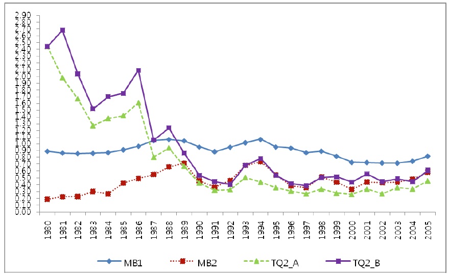
A. Comparison of the Four Estimation Methods: MB1, MB2, TQ2_A, and TQ2_B
In this section, we summarize the four approaches, compare their findings, and propose the best approach for estimating FV. We do not report TQ1 here because TQ1 is not accurate in calculating the market values of preferred stocks, as explained above. Instead, we focus on TQ2 and split it into two methods, namely, TQ2_A and TQ2_B. The four approaches considered here are as follows:
Among the four approaches,
Then, we can say that the estimates by either method,
Of the two methods,
>
B. Comparison between Chaebol and Non-Chaebol Firms
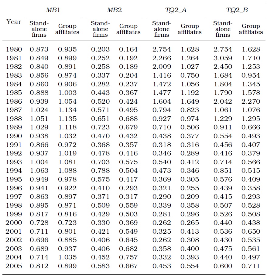
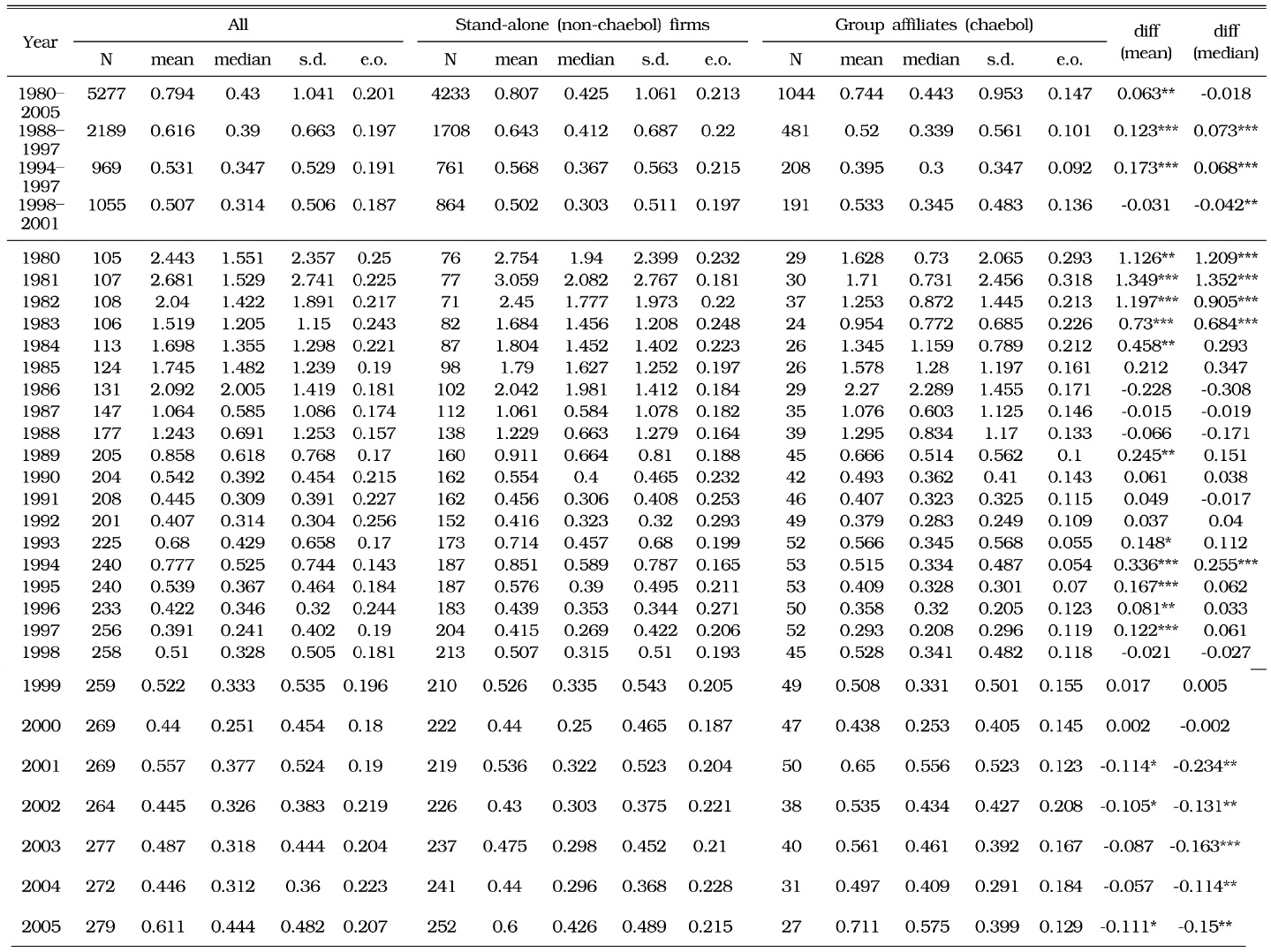
Table 1 compares the values of group affiliates and stand-alone firms across the four alternative methods. Except
[TABLE 1] COMPARISON OF TOBIN Q’S BY APPROACH AND FIRM TYPE

COMPARISON OF TOBIN Q’S BY APPROACH AND FIRM TYPE
Table 2 provides more details about the FV estimates using the
[TABLE 2] ESTIMATION OF TOBIN Q'S OF KOREAN FIRMS (METHOD: TQ2_B)

ESTIMATION OF TOBIN Q'S OF KOREAN FIRMS (METHOD: TQ2_B)
However, after the crisis, when corporate structuring was undertaken to some degree, the mean and median of group affiliates exceeded those of stand-alone firms. Since 2001, the median market value of the group affiliates, using any approach, has been greater at the 1% or 5% significance levels. We attribute this change to substantial improvements in performance and the market value of group affiliates as a result of corporate restructuring. Aside from Tobin’s Q, group affiliates have outperformed stand-alone firms in short-term monthly stock market returns (AR, abnormal returns), long-term rate of return (HPR, holding period return), or rate of operating profits (Lee, Kim, and Lee 2010).
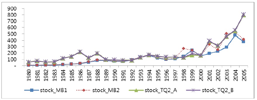
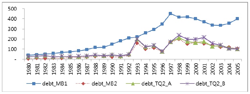
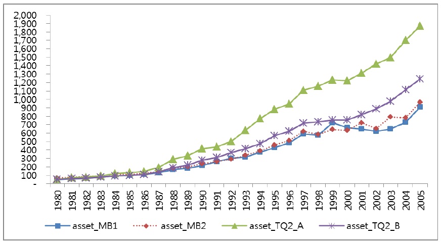
1In Figure 1, the trend of TQ2s shows a strong fluctuation during the long periods. The reasons for this fluctuation are as follows. First, only TQ2s reflect the market value of asset as well as stock and debt of individual firms. Therefore, we can see a rapid downward slope of TQ2s because the measurements reflect the replacement cost of assets using depreciation rate. Second, the Korean economy experienced a fast and high growth rate since the1960s. During these periods, stock value of firms increased rapidly. The trend is indicated in Figure 2-A. After the 1990s, stock value shows a downward slope that reflects the overinvestment of business group affiliates. 2The stock values of MB1 and MB2 refer to the market value of stock from market capitalization at year-end for both common and preferred stocks, respectively. Therefore, the time trend of the two measures must be the same during the periods. However, the trends are different in Figure 2-A, especially in the latter part of the time trends. Figures 2-B and 2-C also indicate a similar pattern. The reason is that samples are different because some samples are dropped as outliers according to the approach. If we compare only the samples with all the four different measurements, we can see the same time trend using the approach. We report the result in the Appendix Figures 2-A, 2-B, and 2-C). 3The economic depreciation rate takes a fixed percentage of the declining balance method. Therefore, depreciation is exponential and has a constant rate of δ.
IV. Experiment on Investment Function Estimation Using All Four Methods
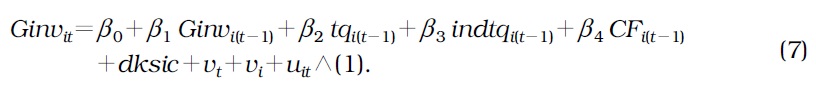
The existing literature uses Tobin’s Q as an important variable in estimating investment function. In this section, we use alternative estimates of TQ to determine how they act as determinants of investment functions. We specify a regression model based on several papers that estimate investment functions, including Scharfstein and Stein (1998), Kim (2002), Carpenter and Guariglia (2003), Hong

The variables in Equation (7) are illustrated as follows:
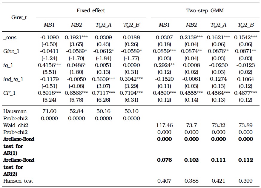
Table 3 shows the estimates of investment function using
[TABLE 3] ESTIMATION OF INVESTMENT FUNCTIONS: BALANCED PANEL (1990-1996)

ESTIMATION OF INVESTMENT FUNCTIONS: BALANCED PANEL (1990-1996)
The above results are telling. First, the
The results for the 2000s or the post-crisis period are different from the results of the 1990s. This finding makes more sense. In other words, in the fixed effect results, the coefficients of
[TABLE 4] ESTIMATION OF INVESTMENT FUNCTIONS: BALANCED PANEL (2001-2005)
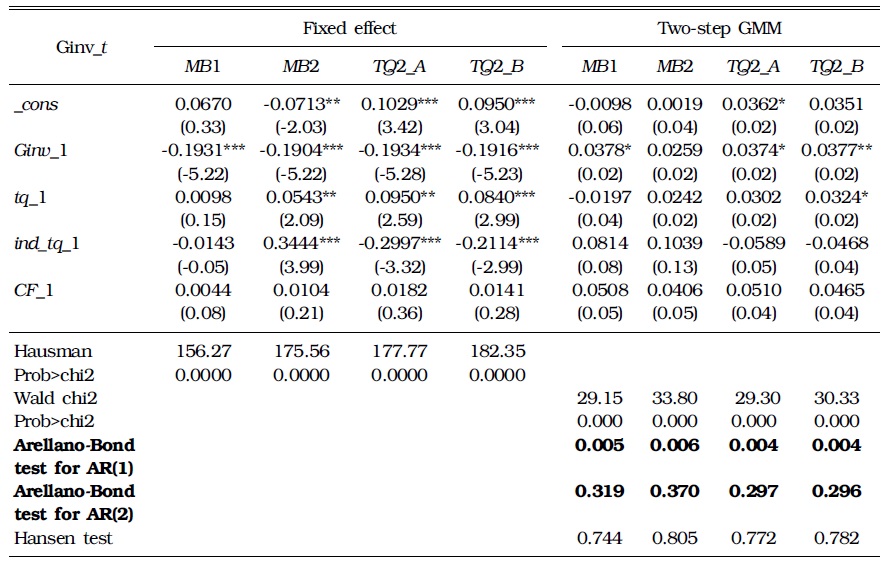
ESTIMATION OF INVESTMENT FUNCTIONS: BALANCED PANEL (2001-2005)
In the 2000s, after the IMF-imposed reform, Korean firms substantially reduced their debts and became more cautious in investment, as verified by Lee, Kim, and Lee (2010) and Choo
4Kim (2010) uses control ownership disparity as an explanatory variable to analyze how the ownership structure affects investment. From the result, he suggests that the ownership control disparity does not affect the corporate decision on investment. 5Other estimators, TQ2_A, and TQ2_B, as well as MB2 satisfy the AR test.
V. Summary and Concluding Remarks
This study uses several approaches to estimate the values of firms in the Korean stock market to find substantially different results depending on the methods
First, the estimates using
As another way to differentiate the reliability of alternative estimates of Tobin’s Q, we conduct the estimation of investment functions. This experiment reveals the weakest reliability of the crude measure or
Given the relative inferiority of
In general, Tobin’s Q is still lower than one, and the average Tobin’s Q of Korean firms is lower than that of American companies (Lee 2013 Ch. 5). This finding implies that a considerable number of the listed manufacturing firms in Korea fail to recover the replacement costs of assets. Further studies should examine what causes this unsatisfactory performance. The question on the presence of the Korean discount, which could have caused Korean firms to be undervalued compared with those in more advanced economies, also remains.