It is a commonly held view in the cognitive sciences that cognition is essentially computation. If this idea is to be explanatorily useful, however, there must be an objective account of when a physical process implements a particular computation. Philosophers such as Hilary Putnam (1988) and John R. Searle (1991) have questioned whether such an account is possible. Searle and Putnam have both claimed that, on a standard understanding of implementation, any reasonably complex physical system implements virtually any computation.1 Chalmers’s account of implementation is specifically intended to refute such claims.
I will argue first that the abstract conception of computation that Chalmers introduces, the combinatorial-state automaton or CSA, cannot be regarded as a full-blown computational model. Although Chalmers may well never have intended it to be regarded in this way, it would provide a more satisfying foundation for an account of implementation if it truly were a general model of computation. I will also argue, second, that the account of implementation in terms of CSAs does in fact allow for trivial implementations similar to those it was introduced to avoid.
1Searle writes: “For any program and any sufficiently complex object, there is some description of the object under which it is implementing the program. Thus for example the wall behind my back is right now implementing the Wordstar program, because there is some pattern of molecule movements that is isomorphic with the formal structure of Wordstar” (Searle 1991, pp. 208-209).
2.1 Implementation of Finite-State Automata
Let us begin with Chalmers’s definition of implementation for a finitestate automaton, or FSA. An FSA with input and output has the following characteristics: A set of internal states
The state-transition function for an FSA determines how the FSA moves from state to state. This definition of implementation requires the corresponding transitions from physical state to physical state in the physical system to be reliably caused. This means not only that a given state
However, Chalmers shows in detail that a more restricted version of Putnam’s and Searle’s conclusion can still be established. I will consider Chalmers’s discussion of this point in the special case of a finite-state automaton without input or output, in part because this is the simplest case and in part because I will make use of this result in my criticism of Chalmers’s own model.
In the case of an FSA without input or output, the state-transition function is simply a function from states to states. Chalmers shows that for any suitably complex physical system that satisfies two simple conditions, we can find a mapping function from states of the physical system to states of the FSA such that the causal relations between the physical states mirror the formal relations between the abstract states of the FSA. The first condition is that the physical system must include what Chalmers calls a “clock.” By this he means simply that a part of the physical system changes reliably from state to state in a non-repeating way, so that each total state of the physical system causes the succeeding state, and no later state is identical with any earlier state. The second condition is that the system has what Chalmers calls a “dial,’’ which simply means that the system has a component that can be in many different states such that when the dial is in a particular state it tends to remain in that state, and the dial states do not affect the operation of the clock. This could be a literal dial or counter (unconnected to anything else), or we could simply treat a system as including marks we could draw on it, for example tally marks.
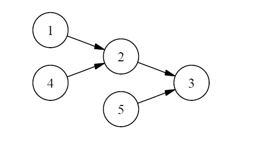
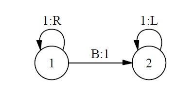
Suppose we now want to construct a physical implementation of the following simple FSA.3

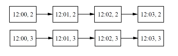
For vividness, our implementation will consist of an actual digital clock with a manually adjustable dial attached to the top. We will set the dial to 1, start the clock at 12:00, and let it run for a few minutes. (For simplicity I assume that time progresses digitally in one-minute increments.) We obtain the following sequence of total physical states of our clock-dial combination:
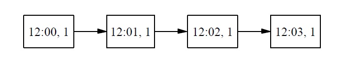
Now, we also know that, if we had set the dial to 2 or 3 instead of 1, the system would have gone through a sequence of states exactly the same as the sequence it did go through, except for the dial setting. So we also have the following counterfactual dependencies:

We can now apply Chalmers’s strategy for constructing a trivial implementation as follows. We will associate each state of the FSA with a set of physical states. We begin with the starting state of the actual run of our physical system, namely the state [12:00, 1], and one of the starting states of our FSA, let’s say state 1. We associate abstract state 1 with physical state [12:00, 1]. According to the state transition function for the FSA, state 1 is followed by state 2, while in the physical system, state [12:00, 1] is followed by state [12:01, 1]. So state 2 is associated with [12:01, 1] and state 3 with [12:03, 1]. We still do not have physical states associated with FSA states 4 or 5. But we want the physical system to have possible states corresponding to these abstract states, and we want counterfactual causal dependencies in the physical system to correspond to the paths through the FSA starting with states 4 or 5. So we next consider what would have happened if the dial had been set to 2. We associate abstract state 4 with physical state [12:00, 2]. Abstract state 4 is followed by state 2, and physical state [12:00, 2] is followed by physical state [12:01, 2], so we need to associate state 2 with [12:01, 2]. State 2 now has two associated physical states: [12:01, 1] and [12:01, 2]. Moreover, as before, state 2 is followed by state 3, so we need to associate state 3 with [12:02, 2]. This second path through the FSA still has left us without a physical state to associate with starting state 5, which leads to state 3, so we associate 5 with [12:00, 3] and 3 with [12:01, 3]. We now have the following associations:
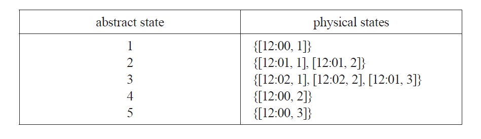
The mapping
Given the mapping from physical states to abstract ones, the clock-anddial physical system meets Chalmers’s criterion for being an implementation of the FSA with which we began.
2.2 Combinatorial-State Automata
It seems obvious that something has gone wrong; it should not be this easy for a physical system to implement a computation. But what exactly is the problem? Chalmers’s suggestion is that an inputless FSA is too simple to provide a model of the kind of computation that underlies cognition. He points out that an FSA with input and output will be somewhat more difficult to implement, but shows that implementations will still be easier to come by than one would like. Again his conclusion is that the model is too simple and unstructured. Chalmers writes: “The real moral . . . is that even simple FSAs with inputs and outputs are not constrained enough to capture the kind of complex structure that computation and cognition involve. The trouble is that the internal states of these FSAs are
Chalmers offers this as a general account of implementation: any abstract computation can be redescribed in terms of CSA state-transitions, so that the above definition of implementation can be applied to any abstract computation whatsoever. Moreover, he argues that the new model avoids the triviality proofs for implementations of finite-state automata.
2Sometimes this is treated as a pair of functions, one from pairs of an input state and an internal state to the succeeding internal state, and one from internal states to outputs. 3To give us something other than a simple straight-line FSA, I have allowed the FSA to have multiple starting states. 4To capture the full power of a Turing machine, the internal states must be allowed to have infinitely many components, but Chalmers considers primarily the finite case.
3. Against the CSA as a Computational Model
There are two ways one might interpret the CSA model. First, it could be intended to be a general model of computation, in the same way that Turing machines or register machines are models of computation. Second, it could be intended, not as a computational model in its own right, but as a convenient formalism for redescribing computations from a variety of specific models, in order to be able to state conditions on implementation in a way that will apply to all of them. I will argue that the CSA cannot play the former role, and that, although it may be able to serve the latter, more modest role, this may not be as advantageous as it first appears.
In many ways the former interpretation of the CSA, as a full-fledged computational model, is a very attractive one. There have been many proposals for making the abstract idea of a computation precise, including Turing machines, register machines, abacus machines, Post production systems, and more. All of these have turned out to be equivalent, in the sense that they can compute exactly the same functions. In another sense, though, they are not equivalent: although a Turing machine and a register machine can each compute, say,
Models of computation typically have two aspects. First, there is an intuitive picture of the essential features of computing, which includes an account of the basic capacities and activities involved in carrying out a computation. These are quite different from one model to the next: the basic capacities in the Turing machine model involve such activities as writing or erasing a symbol and moving to the right or left; the Markov model involves basic activities such as pattern matching and substitution, and so on. Second, the intuitive picture guides the construction of a formal mathematical model. These are quite different from one computational model to the next, but each of them construes a model as a kind of set-theoretic construction, a sequence of parameters whose values must satisfy certain constraints.5 The CSA certainly counts as a model in the sense of a set-theoretic construction. But there is no intuitive conception of computation underlying it. As a result, I will suggest in section 3.1, it does not offer a perspicuous way of explaining or understanding computations. The lack of an intuitive picture underlying the set-theoretic construction may also be the reason that the constraints placed on the model do not yet rule out ``computing’’ the uncomputable, as I will suggest in section 3.2.
3.1 First Problem: Lack of Perspicuity
If we consider how to translate a TM description into a CSA description, we may begin to wonder whether something has gone wrong. Consider the following very simple two-state Turing machine. If started on the leftmost of a string of 0 or more 1’s, it will move to the right, add a 1, and then move back to the left to halt on the first blank space before the 1’s. We could think of it as computing the function
How should this Turing machine be described in the CSA formalism? A state of the CSA will be a vector with components for each square of the TM and a component for the internal state of the TM. To keep things simple, let us restrict our TM to a tape with only three squares. Each square will either be blank or contain a 1, and any combination of blanks and 1s will be a possible state of the tape. This gives us eight possible states so far. States must also have a component to represent the internal state of the TM; since our TM has two possible internal states, we now have 8 × 2 = 16 states. Finally, a CSA state needs to indicate the position of the TM’s read/ write head. The head must be on one and only one square of the tape, so we have a grand total of 16 × 3 = 48 distinct states the CSA can be in.6
In the general case, CSAs may have inputs and outputs as well as internal states. But this is not required to represent a Turing machine. There is no output aside from the final state of the tape. Chalmers suggests that the TM be regarded as having input only once, when it starts, but we can equally well regard it as having no input at all if we treat every state as a starting state, since the input is also simply a distribution of symbols on the tape.
Finally, in addition to state vectors (and input and output vectors if necessary), a CSA must have a state-transition function. Since we do not need inputs and outputs for our TM representation, we can regard this function as simply a function from state vectors to state vectors. A function is simply a set of ordered pairs, so the most obvious way to represent such a function is to list every such pair. Equivalently, we can regard each ordered pair as a state-transition rule stating that its first member must be followed by its second member. Call a description of a CSA by means of such a complete list an
The first thing to notice about this listing is that it seems rather long as a way of characterizing a Turing machine that we could describe very briefly and simply! And of course this is the description for a machine with a tape only three squares long; every additional square of tape will double the number of possible states, so that to represent a machine with a tape of, say, 1000 squares, we will need more than 21000 states, or around 10300, and the same number of state-transition rules in an exhaustive listing.
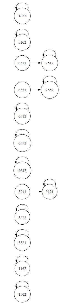
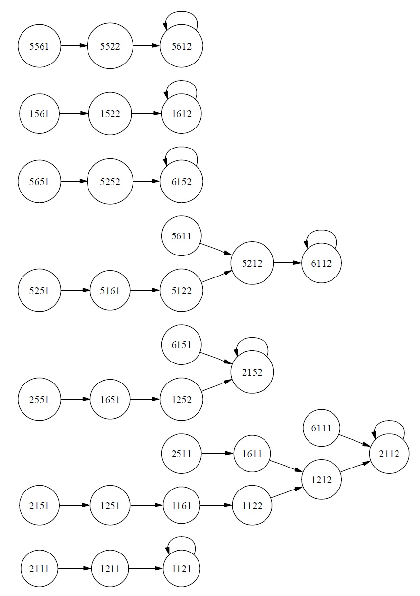
[Table 1.] CSA Transcription of Simple Turing Machine
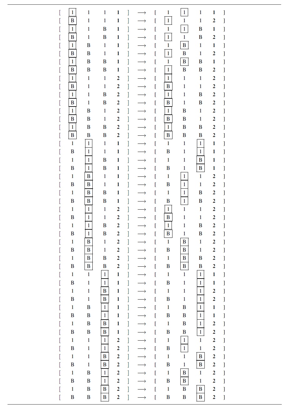
CSA Transcription of Simple Turing Machine
Another way to get a visual impression of the decrease in perspicuity that results from redescription as a CSA is to consider a state-transition diagram. Notice that our CSA transcription of the simple Turing machine has absorbed the Turing machine’s tape into its internal state, so that the CSA has no input or output.7 But this means that in a sense the CSA just
Now, what is the significance of this example? Let us consider two cases, first the case of a finite CSA such as the example we have been considering, and second, an infinite CSA that represents the same TM with an infinite tape. In the finite case it is tempting to say that the CSA does not represent a general algorithm at all in the way that the TM does, because information is actually lost in the redescription of a TM as a CSA. If you extend the tape of the TM, the very same TM description will now characterize a machine that computes the same function over a larger domain. But you cannot deduce from the state-transition function of a CSA how it should behave if we add more substates to represent additional squares of tape. We could say that the state-transition function of the CSA does not determine what mathematical function the CSA is computing. We could try to find the simplest description of the general principles the CSA is applying, and then use those general principles to project how the CSA should behave if extended to represent a larger tape. But the state-transition function itself does not determine this.
If we have an infinite CSA representing our TM with an infinite tape, then we will have all the information we need to determine what mathematical function is being computed. In this case, it may still be reasonable to say that the CSA does not represent an algorithm at all; certainly it does not represent one perspicuously. The information about the TM algorithm is present only in the same way that the laws of motion and gravitation would be present in a complete description of all the possible trajectories of objects in the universe. We have a complete listing of what the TM will do under every possible circumstance, but we have no easy or automatic way to determine the general principles that underlie these actions.
A closely related way to look at the matter is to notice that a state of the CSA that describes the Turing machine represents what Turing called a “complete configuration’’ of the machine, and what is now often called the state of a computation. The state transition rules relate complete computational states, and taken as a whole they specify every possible course the computation could take. So the state transition function in a sense gives us the results of applying an algorithm rather than the algorithm itself.
3.2 Second Problem: Excessive Power
Without unspecified restrictions, CSAs are too powerful to count as a computational model. There are at least two ways to see this point.
First, recall that Turing machines and other computational models were originally introduced to try to provide a precise interpretation of the idea of an effective procedure or algorithm for computing a function. Turing machines (and other models) have the following property: if we can find a Turing machine that computes a given function, then we have found an effective procedure for computing the function, and the TM description is a description of this procedure. But this is simply not true for CSAs in general. There will always be a CSA which finds the value of a function for any argument in some finite range in a single step. For instance, in the case of the function
Second, consider the case of a CSA whose states have an infinite number of components. Chalmers explicitly allows this, as indeed he must if it is to be possible to have a CSA transcription of a TM with an infinite tape.9 But now the state-transition function will need to be able to take infinitely many arguments (so that an exhaustive listing would have infinitely many state-transition rules). But once we allow the state-transition function to have infinitely many arguments, it is hard to see how to prevent CSAs from being able to “compute” functions that are in fact not computable! And clearly a model that permits “computation” of uncomputable functions is not a good candidate for a model of computation.10
I hesitate to place too much weight on this point, since Chalmers only briefly mentions infinite CSAs, and he does state that “restrictions have to be placed on the vectors and dependency rules, so that these do not encode an infinite amount of information” (Chalmers 2011, p. 330). Chalmers does not state what these restrictions might be, however. Clearly
In some ways the most natural way to limit the class of CSAs to those that compute functions that are “computable” in the usual sense might be to require that there be a way to give a finite specification of the state-transition function. More precisely, it would be natural to require that the statetransition function be
The problem of excessive power can be put in another way. Traditional computational models begin with a highly restricted set of abilities, and then show that more and more complex tasks can be performed by combinations of these basic abilities. It is precisely the fact that complex tasks can be accomplished by complex applications of simple abilities that shows that the tasks are computable. However, the CSA model in a sense moves in the exact opposite direction. It begins with the ability to move from absolutely any state to absolutely any other state, so that to guarantee that only computable functions can be captured, we have to impose restrictions.
3.3 Third Problem: Trivial Implementations
The principal advantage of the CSA over the FSA is intended to be that CSAs are not similarly susceptible of trivial implementations, such as the implementations consisting of a clock and a dial considered earlier. Of course, a finite CSA is equivalent to an FSA, as Chalmers himself points out. In fact the state-transition diagram displayed earlier can be construed as that of an inputless FSA. Chalmers’s own argument, reviewed earlier, shows that there is a trivial implementation of this inputless FSA by means of a clock and a dial. However, as Chalmers points out, “the
However, if we adopt Chalmers’s official definition of implementation for a CSA, without any additional restrictions, it is possible to implement a finite, inputless CSA in a physical system in which there is almost no causal interaction at all between the subcomponents of the system. Consider the following simple modification of Chalmers’s technique for finding trivial FSA implementations. Instead of implementing the CSA with a single clock and dial, we will implement a CSA whose states have
This gives us physical implementations for total states of the CSA, but we have not yet specified physical implementations for the individual components of those states. Indeed, it may seem backward to find implementations of the total state first, since the total abstract state is a vector of abstract substates, and we would like its physical implementation to similarly be a vector of physical states. However, once we have the physical implementations of total CSA states, we can easily construct the implementations of their substates. We can specify the grouped physical state type which implements (maps to)
Of course, this mapping of physical states to substates of the CSA generates a lot of new theoretical ways to physically implement a given CSA state. However, given the physical impossibility of the clock and dial settings of the physical substates differing from one another, only a small number of the many theoretically possible implementations of a given total CSA state will actually be physically possible. Indeed, every physical implementation of
What makes such trivial implementations possible is in part the fact that Chalmers’s official definition of implementation appeals only to transition rules that link total states, not to more local or general rules; and in part the fact that in the physical system I propose it is impossible for the dial and clock readings of the various physical substates to differ from one another. One might wonder whether this latter point somehow disqualifies the implementation. But there doesn’t seem to be anything in the official definition of CSA implementation which rules out this sort of causal connection between the physical substates of the overall system, and it is not clear what constraint one might add to rule it out. There cannot be a general prohibition on causal connections between subcomponents, since we
My first two criticisms of the CSA model focused on the abstract model itself, emphasizing the need for additional constraints on this abstract model. My guess is that the way to avoid trivial implementations, however, is different. Chalmers describes the root idea of his account of implementation as the idea that there is an isomorphism between “the formal structure’’ of the abstract computation, and “the causal structure’’ of the physical system that implements it.11 We normally think of implementation as a relation between abstract structures and concrete physical processes. But of course
5I am drawing here on R. Gregory Talor’s helpful section “What is a Model of Computation?” (Taylor 1998, pp. 342-344). Taylor suggests that the existing models of computation are so varied that is no core of essential features common to them all: “the most that can be said is that the various models ... exhibit cetain family resemblances” (Taylor 1998, p.344). 6The simplest way to represent the position of the head would be to add another component to the state vector and use it to indicate the number of the square on which the head is located. But this would not work if we allowed infinite vectors, which we need to fully represent a TM. Chalmers suggests letting the components for squares of the tape be ordered pairs of a symbol and a yes/no value indicating whether the head is on the square. If we do this we need to add a restriction specifying that only one square can have the value “yes.” In my state-transition table below I depict the position of the head pictorially without worrying about the precise set-theoretic representation of this information. 7We saw earlier that we do not even need input at the first step if we regard the CSA as having multiple starting states. 8The node labels require some explanation. Each digit represents a separate component of the CSA state. The first three digits represent the three squares on the tape. For these digits, ‘1’ means there is a one on the square and the head is not in that position; ‘2’ means there is a one on the square and the head is positioned at that square; ‘5’ and ‘6’ represent a blank without and with the head, respectively. 9It is often pointed out that a TM tape need not actually be infinite, but may only be unbounded. But it won’t do to simply give a CSA an unbounded number of states, since this would make the state-transition rules impossible to specify. This is another symptom of the fact that TM rules are general in a way that CSA statetransition rules need not be. 10A closely related observation is that without further restrictions, a diagonalization argument will show that the CSA has nondenumerably many possible states. 11As Cocos (2002, p. 44) stresses, the definite description “the causal structure’’ is misleading, since (as Chalmers recognizes) the same physical system will have many causal structures.
4. The CSA as a Transcription Device
I have argued that the CSA does not constitute a computational model in its own right, at least as presently described. (It is possible that a revised version with restrictions imposed on the allowable states and transitions might be.) It is entirely possible, however, that it was not Chalmers’s inten-tion to provide such an account. It may be that he intends the second interpretation mentioned above, construing the CSA merely as a convenient formalism into which more specific abstract machines can be translated.
If this were the case, then, since each TM state-transition rule (for instance) corresponds to a large number of CSA state-transitions (in fact an infinite number if we are representing a TM with an infinite tape), we could abandon the exhaustive listing as a way of characterizing a CSA, and translate each TM rule by a universal quantification over CSA states. Some sentences in “Rock’’ appear to suggest something like this: Chalmers mentions that “often the state-transitions of a CSA will be defined in terms of
For the example we have been considering, we could say that the function that maps a state
If we took this approach, then constructing informative descriptions of rules underlying the state transition function would be straightforward, since they would simply transcribe the general rules guiding the more specific abstract machine. We could be sure that we were considering only CSAs representing computable functions, since they would all be transcribed from models which guarantee computability. But we would entirely lose the attractive idea of the CSA as a model that represents the concept of computability in a completely general way.
Moreover, once we lose the idea that a physical system implements a computation if and only if there is a CSA that implements it, it becomes less clear what the advantage of using CSAs to define implementation is. For on this more limited understanding of the significance of the CSA, we will need to decide how to translate each more specific computational model into a CSA, a task which may prove to be just as difficult as defining implementation directly for each specific model.
12n is the number of squares on the TM tape — three, in the case we have been considering. This description treats the first n components of the state vector as representing the states of the tape’s n squares, the next component as representing the index of the square the head is currently over, and the final component as representing the current internal state of the TM.
It would be satisfying to have a general account of computation, an account fine-grained enough to distinguish between different kinds of implementation of computations of the same function, and general enough that it can describe any abstract computation.13 It is possible that when Chalmers provides details that were only hinted at in his earlier papers, in particular about the restrictions that need to be placed on allowable CSA states, the CSA will in fact turn out to be such a model. But it cannot yet be regarded in that light.14
13One proposed model of this sort is Yuri Gurevich’s Abstract State Machine: see e.g. Dershowitz and Gurevich (2008). 14This paper is a revised and expanded descendant of “Implementation and Indeterminacy,’’ in J. Weckert and Y. Al-Saggaf, eds.,