Consciousness is a significant research topic in philosophy and a variety of theories and elaborate thought experiments have been put forward. However, although a great deal of effort has been expended, it can be argued that our understanding of consciousness has failed to advance much beyond Descartes. The situation has changed in recent years with the emergence of the scientific study of consciousness. This aims to gather data about correlations between consciousness and the physical world while suspending judgement about the metaphysics and philosophical debates. Scientific data about the correlates of consciousness could help us to improve our philosophical theories about consciousness and it has many practical applications - for example, it could help us to answer questions about the consciousness of brain-damaged patients, infants and animals.
In an experiment on the correlates of consciousness, the general procedure is to measure consciousness, measure the physical world and look for a relationship between these measurements. The measurement of consciousness relies on the working assumption that consciousness is a real phenomenon that can be reported verbally (“I see a red hat”, “I taste stale milk”) or through other behaviour, such as pushing a button, pulling a lever, short term memory (Koch 2004) or the Glasgow Coma scale (Teasdale and Jennett 1974). The assumption that consciousness can be measured through behaviour enables us to obtain data about it without a precise definition. However, this reliance on external behaviour limits consciousness experiments to systems that are commonly agreed to be conscious, such as a human or a human-like animal. It is not possible to carry out this type of experiment on non-biological systems, such as computers, because a computer’s reports are not generally regarded as a measurement of consciousness (Gamez 2012).
The physical world is measured to identify spatiotemporal structures that might be correlated with the measurements of consciousness. In this paper I am focusing on the correlates of consciousness in the human brain, 1 which will be defined in a similar way to Chalmers’ (2000) definition of the total correlates of consciousness:
Correlates defined according to D1 would continue to be associated with consciousness if they were extracted from the brain or implemented in an artificial system. ‘Spatiotemporal structures’ is a deliberately vague term that captures anything that might be correlated with consciousness, such as activity in brain areas, functions, neural synchronization, computations, information patterns, electromagnetic waves, quantum events, etc.
In an experiment on the correlates of consciousness a contrastive methodology is typically used that compares the state of the brain when it is conscious and unconscious, or compares conscious and unconscious states within a single conscious brain - for example, using binocular rivalry (Logothetis 1998) or through the subliminal presentation of stimuli (Dehaene et al. 2001). 3 Systematic experiments are needed to test all possible combinations of spatiotemporal structures that might form CC sets (see Table 1). When one or more CC sets have been identified they can be used to make predictions about the level and contents of consciousness, which can be compared with first person reports.
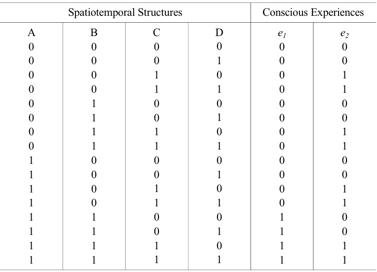
Illustrative example of correlations that could exist between conscious experiences (e1 and (e2 ) and a physical system. It is assumed that (e1 and (e2 can occur at the same time. A, B, C and D are spatiotemporal structures in the physical system, such as dopamine, neural synchronization or 40Hz electromagnetic waves. A, B, C and D are assumed to be the only possible features of the system. ‘1’indicates that a feature is present; ‘0’ indicates that it is absent. In this example D is not a correlate of consciousness because it does not systematically co-vary with either of the conscious states. {A,B} is a set of spatiotemporal structures that correlates with conscious experience (e1 . {C} is a set of spatiotemporal structures that correlates with conscious experience (e2 .
While most scientists have focused on the neural correlates of consciousness, there are several different types of spatiotemporal structure in the brain that could form CC sets. For example:
If H1 is correct, it will be possible to create artificial consciousness by running a computer program. We could also create a copy of our consciousness by running a program that simulates our brain at an appropriate level of detail. The consciousness associated with these programs would be the same regardless of whether they are running on a modern desktop computer or on Babbage’s Analytical Engine.
This paper examines whether H1 could be scientifically tested using the same methodology as an experiment on the neural correlates of consciousness. This could be done by measuring the computations in the conscious brain, measuring the computations in the unconscious brain and looking for computations that are only present in the conscious brain. 6 The difficulty with this type of experiment is that very few methods for measuring computations in physical systems have been put forward.
Modern digital computers execute programs and convert input strings into output strings, and it might be thought that we could identify computations in other physical systems by looking for executing programs or string processing (Piccinini 2007). The limitation of this approach is that it is unlikely to be applicable to the brain, since it is far from obvious that the brain’s operations are based on programs or string processing. If we want to test the hypothesis that the brain contains computational correlates of consciousness, we will have to find a more general way of measuring computations that can be applied to a wide range of physical systems.
A second way of measuring computations in a physical system is to map the computation onto a finite state automaton (FSA) and determine whether the sequence of states of the FSA over a particular execution run with a particular input pattern matches the sequence of states of the target system. FSAs are often used to specify programs’ state transitions and they can be used to identify computations in a wide range of systems, including the brain. The problem with FSAs is that a disjunctive mapping can be used to interpret a sequence of unique states in
The most promising method that I am aware of for identifying computations in physical systems is the combinatorial state automata (CSA) approach put forward by Chalmers (1996;2011), which can be roughly summarized as follows:
CSAs are related to FSAs, but more restricted in the systems that they apply to. This might enable them to identify computations in the conscious brain that are not present in the unconscious brain. CSAs are also more general than accounts of implementation based on modern digital computers. While many criticisms have been made of Chalmers’ account of implementation (Scheutz 2001; Miłkowski 2011; Ritchie 2011; Brown 2012; Egan 2012; Harnad 2012; Klein 2012; Rescorla 2012; Scheutz 2012; Shagrir 2012; Sprevak 2012), it is far from clear what could be used to replace it if it was found to be seriously flawed (see Section 4).
Chalmers’ account of implementation enables us to replace the general hypothesis that there are computational correlates of consciousness (H1) with a more concrete hypothesis that could potentially be tested:
We can test H2 by measuring consciousness through first person reports, measuring CSAs in the brain (see Section 3.1) and looking for correlations between these two sets of measurements. This type of experiment must meet at least two requirements:
This paper will examine whether the potential correlation between CSAs and consciousness could be experimentally tested in a way that is consistent with these requirements. To make the issues clearer I will focus on a simple test system, a desktop computer running a robot control program, which is described in Section 2. If Chalmers’ method could successfully identify the computations in this test system, then we would have grounds for believing that it could be used to identify computations in the brain. Section 3 raises a number of problems that occur when we try to use Chalmers’ method to identify computations in the test system in a way that is consistent with R1 and R2. These suggest that a CSA-based account of implementation cannot be used to identify computational correlates of consciousness in the brain. The discussion in Section 4 considers whether the problems with Chalmers’ approach could be addressed by developing a better way of measuring computations in physical systems.
1I am focusing on the human brain because we are confident that it is linked to conscious states. Once we have identified the correlates of consciousness in the human brain we can use them to make predictions about the consciousness of other systems (Gamez 2012). 2In D1 CC sets are linked with individual conscious experiences. To improve the readability of the text I will often talk about the correlates of consciousness in general, which can be considered to be the complete set of CC sets. 3Reviews of some of this experimental work are given by Rees et al. (2002), Tononi and Koch (2008) and Dehaene and Changeux (2011). 4Some of the difficulties with experiments on information integration and consciousness (Gamez 2014) also apply to experiments on the computational correlates of consciousness. 5A real world program or computation can be decomposed into collections of subroutines, calls to external libraries and the operating system, etc. In H1 all of these computations are considered to be the single computation, Cc . 6To prove that computations are sole members of CC sets it will also be necessary to demonstrate that the substrate or mechanism by which the computation is being executed is irrelevant. A discussion of this issue is given in Gamez (2012).
Before Chalmers’ CSA-based account of implementation is applied to the brain it is advisable to check that it is a good way of identifying computations in a much simpler physical system. This can be done by applying Chalmers’ approach to a basic test system that has known computations. If the result matches the computations that we expect to be executing in the test system and is consistent with R1 and R2, then the same approach could potentially be used to identify computational correlates of consciousness in the brain.
The test system that I have selected for this purpose is a standard desktop computer running a robot control program. Since this is a paradigmatically computational system, we would expect that the CSA corresponding to the running program will be easy to identify using Chalmers’ method. The use of a paradigmatically computational system as a test system also avoids contentious discussions about whether arbitrary physical systems, such as walls, rocks or buckets of water, can be said to implement a particular computation (Searle 1990; Copeland 1996). Most people would agree that a desktop computer running a particular program is a computational system and that it is implementing the computations listed in the program. A third reason for choosing this test system is that our theories of mind are often influenced by our beliefs about how computers work. These theories could be clarified and improved by developing a better understanding of the relationship between a physical computer, the programs running on the computer and the computations that the computer is executing.
The test system is presented in detail to support the discussion and to enable other people to suggest how it could be analyzed for computational correlates of consciousness. Although it is not capable of any of the functions that have been proposed to be linked to consciousness (for instance, the implementation of a global workspace (Baars 1988)), the issues raised in this paper are applicable to any program that could run on a computer. No claim is being made about whether or not the test system is actually conscious –it is just being used to illustrate how computations could be identified in a way that is consistent with the requirements of an experiment on the correlates of consciousness (R1 and R2). 7
2.2 Desktop Computer, P1 and the Simple Robot
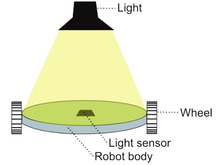
The test system is a standard desktop computer that controls a simple two wheeled robot (see Figure 1). I have chosen a robotic system to address claims that embodiment is necessary for cognition and/or consciousness. The robot has a light sensor on top, and the motors driving the wheels can be independently controlled. This system is detailed enough to enable questions about the physical implementation of computations to be accurately posed, but hopefully simple enough so that the discussion does not get bogged down in details about drivers and internal communications.
The code for the control program,
Under the control of this program the robot will move forward in a straight line when the light is changing, or circle if the light stays the same. A stroboscope with double the while loop’s frequency will be required to drive the robot forward. The robot would exhibit smoother behaviour if the
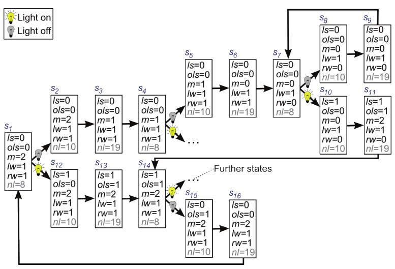
The CSA description of the program,
The CSA that corresponds to a program will in most cases be an
7Also requirement R3, which is set out in Section 3.1.
3. Can CSA1 be identified in the Test System a way that is Consistent with R1 and R2?
Since the test system is a paradigmatic example of a computational system, we would expect it to contain a clearly defined set of computations that could easily be identified with Chalmers’ method. It also seems reasonable to expect that the CSA corresponding to the executing program could be unambiguously identified in the test system. After discussing the approach that I will use to analyze the test system in Section 3.1, I will highlight some of the problems that occur when we try to use Chalmers’ method to analyze the test system for computations in a way that would be consistent with an experiment on the correlates of consciousness.
3.1 Method for Identifying CSAs in the Test System
The programs that are executing on the test system can be identified by launching the Task Manager in Windows or by typing “ps –el” in a Linux shell. If
Instead, the CSAs in the test system will be identified by mapping what Chalmers (2011, p. 328) calls the “distinct physical regions” of the system (if such distinct regions can be found) onto CSA substates. By observing how these regions change over time we can map out the state transitions and their conditional structure, which enables us to identify the CSAs that are executing in the system. This method for measuring CSAs is summarized as the following requirement:
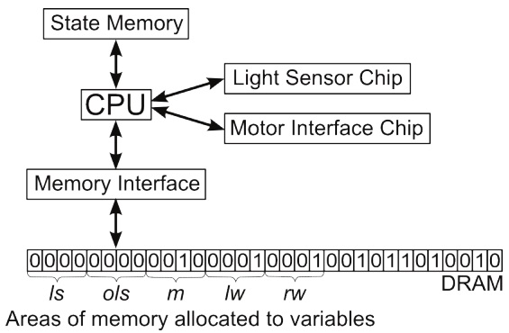
This method can be used to infer the brain’s CSAs from measurements of neuron voltages, blood flows, glia activity, and so on. The test system can be analyzed in a similar way by treating it as a physical object made of silicon, copper, plastic, etc., and mapping its distinct physical regions (for example, DRAM storage cells – see Section 3.3) onto CSA substates. While some facts about a computer’s operation will be used to illustrate the CSA mapping problems, the analysis should not depend on prior knowledge about the operating system or variable encoding, and the person doing the analysis will not be able to connect up a keyboard and screen to get the computer’s own ‘view’ of its internal states.
If the test system is implementing
It might be thought that we could solve this problem by mapping substates of
These problems linked to virtual memory and CPU caching are likely to defeat simple methods of interpreting the test system as an implementation of
Since virtual memory and CPU caching are non-essential optimization strategies, they will be set aside for the rest of this paper and the test system will be revised so that
3.3 Mapping Physical States onto CSA Substates
The most obvious ‘distinct physical regions’ of the simple computer are the DRAM storage cells. Since the person analyzing the simple computer does not have high level information about the operating system (for example, whether it is 32- or 64-bit) 8 - there are no restrictions on how they should organize these cells into higher level groups. This leads to an extremely large number of equally valid ways of interpreting the simple computer’s DRAM storage cells as substates of a CSA.
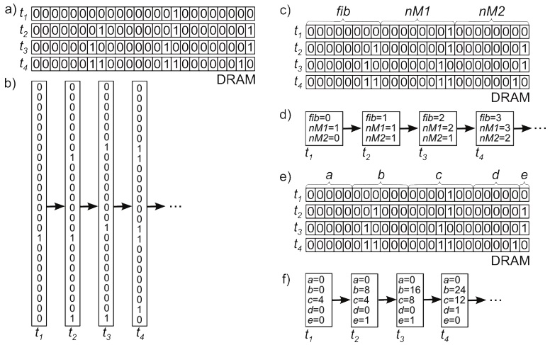
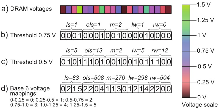
The voltage in a DRAM storage cell typically ranges from 0 to 1.5 V and changes continuously with time (typically decreasing between refresh cycles). To begin with I will consider the standard way of interpreting a DRAM voltage, which is to apply a threshold and interpret a voltage above the threshold as a ‘1’ and a voltage below the threshold as a ‘0’. To make the discussion clear, I will use a simpler example than the test system: a C++ program,
When
If we want to locate the CSA corresponding to
All three CSAs in Figure 4 are equally valid mappings of physical states of the computer onto CSA substates, and the substates within each CSA are causally related to each other to the same extent. This is because the number of bits that are allocated to each number is not a ‘distinct region’ of the physical system, but a high level piece of information that is typically accessed through a graphical interface. There is no canonical way of mapping groups of DRAM cells onto CSA substates, and so when the simple computer is running
So far I have assumed that the voltages are mapped onto 1s and 0s in the standard way. However, an external observer who was attempting to analyze this system for CSAs would not be constrained to apply any particular threshold to this voltage, and the mapping between voltage values and substate values could be carried out in many different ways – for instance, 1.5 V can be interpreted as a substate value of 1, 100 or -0.75. The sampling frequency and the way in which the system is divided into discrete spatial areas also have major effects on the substate values. 10 Some of these problems are illustrated in Figure 5.
While Chalmers acknowledges that a system can implement more than one computation, he claims that this is not a problem as long as it does not implement every computation. However, to prove that a CSA is correlated with consciousness we have to show that it is executing when the system is conscious and
3.4 The Causal Structure of a Computer
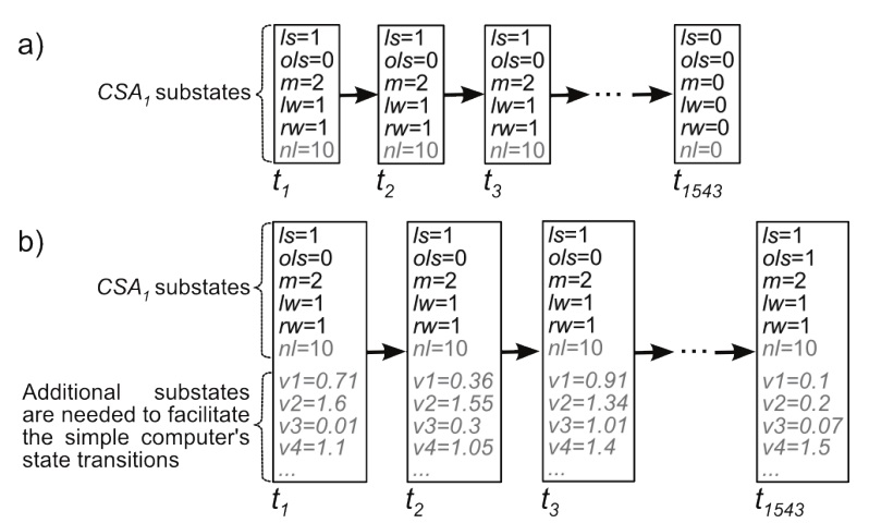
Suppose that we ignore the problems raised in the previous section and map the substates of
The state transitions in the simple computer depend on complex causal interactions between the DRAM voltages and a large number of substates in the CPU and the rest of the system (Figure 6b). 11 These electromagnetic interactions between voltages in different parts of the chips are governed by complex laws, and the number, type and behaviour of the additional substates varies with the architecture of the computer. Since these additional substates are not specified in
This breaks the link between the program that is running on a computer and the CSAs that are present in the physical states of a computer. While it is possible that
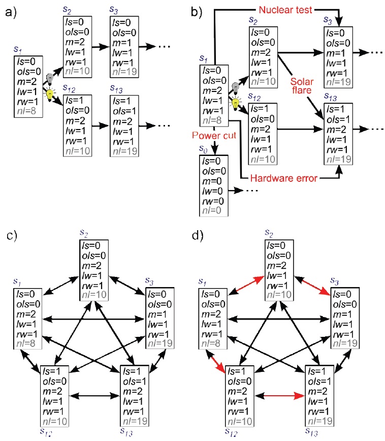
A real physical system is subject to influences from its environment that cause state transitions. While great care is taken to isolate computers’ electronic components, they are still subject to external interference, which can cause them to make state transitions that are not specified in the program. A computer executing
The causal topology of a physical system at a particular point in time includes all of the possible state transitions that
When a computer’s state transitions do not follow the program or operating system, we typically say that the program or computer has crashed or failed. However, the analysis described in this paper is solely based on an examination of a system’s states (R3), and in this context there is no crashing or failing – just state transitions that are or are not conditional on external events. All of a system’s possible state transitions count for its implementation of a CSA – any implications that these might have for the user’s interaction with the computer are irrelevant.
This problem with a CSA-based approach to implementation has been considered by Chalmers (2012), who suggests that some form of normal background conditions might have to be included: “... the definition might require that there be a mapping M
If a plausible account of normal background conditions cannot be developed, then the only CSAs that are actually implemented by humanscale physical systems, such as brains and computers, are ones that have complete connectivity between their states. Human-scale physical systems cannot be completely isolated from low probability events, such as electrical interference or solar flares, that counterfactually link each state of a CSA to every other state. As systems get larger, the external factors that could cause state transitions will decrease, and the universe as a whole does not have a completely connected state structure because there is no possibility of outside interference.
It might still be claimed that a system is implementing
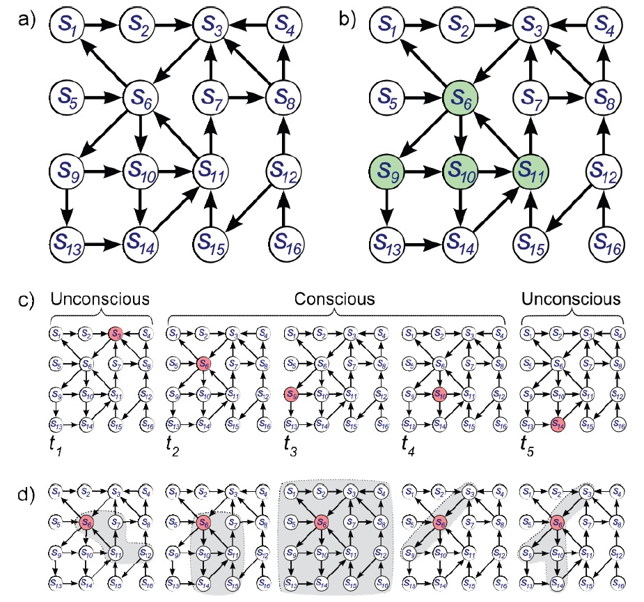
Consider a simplified ‘brain’ (SB) that consists of four biological neurons, each of which can be in two states, firing or not firing. The complete state space has 16 different states,
Suppose that SB enters state
It might be objected that in this example states
The problem with this claim is that a person who was monitoring the physical system would have no reason to believe that a particular sub-CSA was being executed or that there was a transition between active sub-CSAs. Nothing in the physical system corresponds to this change - someone who only knew the physical facts could not identify or predict it. It is only because there is a change in the consciousness associated with the system that we are inclined to say that one sub-CSA is being executed instead of another. This suggests that a change in the executing sub-CSA is not a measureable property of the physical system, but is being attributed to the system to support a particular theory – namely that executing CSAs are linked to conscious states. A correlate of consciousness is a property of the physical system that is correlated with the presence of conscious states – we measure the physical system, measure consciousness and look for correlations between the two. Consciousness cannot be used to identify features of the physical system that are supposed to be correlated with consciousness – an independent measure of a physical property is required. The state and the set of CSAs that overlap a state might be considered to be objective facts about a system (if one could address the other problems with CSAs that have been raised in this paper). It is not a fact that a single CSA is being executed to the exclusion of all the other CSAs that overlap the current state.
In systems with more than a few elements an extremely large number of CSAs will overlap each state. This number increases factorially with the size of the system, which will rapidly make it impractical to record the CSAs that are correlated with consciousness. A second issue is that any small change to the system’s state space will alter some of the CSAs that overlap a particular state. So even if was possible to exhaustively list the CSAs that were correlated with consciousness in one system, this list would become obsolete once the system changed its state space, which happens all the time in the brain. It would also be difficult or impossible to use the sets of CSAs that are correlated with consciousness in one system to make predictions about consciousness in other systems.
Given these problems it is more plausible and experimentally tractable to focus on correlations between particular states of a system and consciousness. In SB it is far simpler to enumerate the states that are correlated with consciousness (
Chalmers’ account of implementation relies on causation to avoid problems with panpsychism and trivial implementations:
If the target system matches the
Chalmers’ vague handling of causation is linked to his use of CSAs to specify causal topologies: “...the CSA formalism provides a perfect formalization of the notion of causal topology. A CSA description specifies a division of a system into parts, a space of states for each part, and a pattern of interaction between these states This is precisely what is constitutive of causal topology.” (Chalmers 2011, p. 341). While a CSA does specify a division of a system into parts and a space of states for each part, it does not
Within the literature on causation, there is a useful distinction between a
While conceptual accounts of causation are unlikely to lead to an agreed fact of the matter about the causal topology that is implemented by a particular physical system (R1), empirical accounts do enable causal topologies to be precisely specified. They also support the identification of supervenient causal relationships at different levels of a system - for example, an empirical account of causation can easily deal with the fact that causal relationships between neuron voltages supervene on ions moving across a cell membrane. This suggests that Dowe’s approach could be used to provide a detailed specification of the amount and type of causal interactions in a system - defining substates as causal processes and linking state transitions to the exchange of conserved quantities, such as mass-energy or momentum. While this would go a long way towards tightening up Chalmers’ account of implementation, it would also virtually eliminate the idea that one system can implement the causal topology of another. Systems with different architectures and materials have very different patterns of exchange of conserved quantities. A modern digital computer, the ENIAC and Babbage’s Analytical Engine that are running the same program will not be implementing the same computations, if this more causally accurate theory of implementation is used to identify the computations. All of the generality of Chalmers’ account will have been lost.
8Roughly speaking, a 32-bit operating system uses a maximum of thirty two 1s and 0s to represent a number or a memory address. A 64-bit operating system uses up to sixty four 1s and 0s to represent a number or a memory address. 9This is because a DRAM cell only holds a single 1 or 0, whereas the P2 variables are encoded using multiple 1s and 0s. 10The application of an arbitrary voltage threshold could be avoided by mapping the DRAM voltages onto continuous substate values. This possibility is discussed by Chalmers (2011, p. 347-349). This would break the link between digital programs and the CSAs implemented by the physical computer and there would still be ambiguities about which parts or aspects of a physical system are measured to extract the analogue values (Gamez 2014). 11The operations and instructions that are carried out by a CPU (AND, OR, etc.) are high level descriptions of the physical circuits, whose electromagnetic interactions cause the state transitions.
This paper has asked whether the execution of a computation could be a sole member of a CC set (H1). In other words, could the execution of a computation be correlated with consciousness independently of the architecture of the system or the material in which it is executing? I have suggested that this question could be addressed experimentally by identifying the computations that are executing in the conscious and unconscious brain. This requires a way of measuring computations in the brain and Chalmers’ CSA approach was selected as the best method that is currently available for this purpose. H1 was then rephrased as the question about whether a CSA could be a sole member of a CC set (H2). To answer this question I investigated whether CSAs could be unambiguously identified in a computer in a way that would be consistent with an experiment on the correlates of consciousness (R1-R3). The following problems were identified:
These problems have been illustrated on some simple systems and they will be many orders of magnitude harder on the brain, which has vague ‘distinct physical regions’ and an extremely large state space that changes all the time. The issues can be separated into theoretical problems (points 3 and 5) and pragmatic difficulties (points 2 and 4). The theoretical problems suggest that CSAs cannot be used to identify computational correlates of consciousness in the brain, even in principle. If the theoretical problems could somehow be addressed, the pragmatic difficulties are likely to prevent us from ever using CSAs to test H1.
The most obvious way of addressing these problems would be to develop a better account of implementation. Chalmers’ theory was not designed for experimental work on the correlates of consciousness, and so it is not surprising that it is does not perform well in this context. Some of the difficulties with the CSA approach are linked to its abstractness and generality, and so it might be possible to fix it by specifying causal topologies in more detail. However, if the CSA account is supplemented with more details about the patterns of exchange of physically conserved quantities, then it will become a description of a physical correlate of consciousness, because it is unlikely that a detailed pattern of exchanges could implemented in different physical systems. It might be thought that the problems of complete connectivity highlighted in Section 3.5 could be fixed by specifying probabilities for each state transition. However, this is unlikely to work in the brain where the state transitions change all the time as the brain learns and shifts between tasks. There does not appear to be an easy way of adding detail to the CSA account that could address the problems that have been identified.
A second way of tackling these problems would be to define computations in terms of their inputs and outputs. For example, an adding function is defined by the fact that it returns the sum of a set of numbers – the details of its implementation do not matter and it would be superfluous to specify it using a CSA. The problem with this approach is that we often exhibit very little external behaviour when we are conscious – for instance, when I sit quietly in an armchair with my eyes closed there is no obvious external behaviour that could be used to identify computations that could be correlated with my consciousness. We might divide the brain up into modules and attempt to specify the computations that are carried out by each module by using their input-output relationships. But many of the computations linked to consciousness are likely to be impossible to partition in this way. Some functions that might be correlated with consciousness are implemented by highly modular brain areas – for example, V5 is linked to our visual experience of motion. But others, such as a global workspace (Baars 1988), are likely to be dynamically implemented through coordinated interactions between many areas of the brain. Since there are an infinite number of ways of dividing up the brain into modules, it is going be very difficult to develop a workable method for defining computations based on the external behaviour of brain areas.
It might be claimed that
The disconnect between a computer’s running programs and the CSAs that it is implementing has implications for the suggestion that we might eventually be able to upload our brain onto a computer or replace part of our brain with a functionally equivalent chip(Moor 1988; Chalmers 1995; Kurzweil 1999; Chalmers 2010). Suppose we manage to identify a CSA in the brain that is correlated with consciousness, write a program that implements this CSA, and run it on a computer. The arguments in sections 3.2 and 3.4 suggest that this system is unlikely to have the same consciousness as the original brain because the CSAs that are present in the computer are unlikely to correspond to the CSAs of the running programs. A computer running a program that simulates my brain is unlikely to be implementing the CSAs that are present in my brain. A chip that replicates the input-output functionality of part of my brain (for example, a silicon hippocampus) is unlikely to be implementing the CSAs of the original brain area. It might be possible to design a different type of ‘computer’ to implement CSAs, but this would require a very different architecture from a standard computer. For example, neuromorphic chips (Indiveri et al. 2011) that use the flow of electrons in silicon circuits to model the flow of ions in neurons might be capable of implementing some of the CSAs that are present in biological neurons.
Many of the issues with experiments on the computational correlates of consciousness will be encountered by experiments on the functional correlates of consciousness. To prove that there are functional correlates of consciousness we need to measure the functions that are executing in the brain, so we can show that certain functions are only present when the brain is conscious. The problems identified in this paper suggest that CSAs will not be a workable method for specifying and identifying functions, and it is not obvious how else one could measure functions during this type of experiment.
The theoretical and pragmatic problems raised in Section 3 suggest that H2 cannot be experimentally tested. While H2 might be a valid philosophical or metaphysical theory about the world, if it cannot be falsified, it is not a scientific hypothesis (Popper 2002). H1 cannot be tested until a plausible method for measuring computations has been found. Many of the problems with Chalmers’ approach are likely to be encountered by other methods of measuring computations, but it will not necessarily be impossible to develop a method that can circumvent these difficulties and meet the requirements of an experiment on the correlates of consciousness (R1-R3). Until such a method has been found, we are likely to make more progress by focusing on patterns in particular physical structures that could be correlated with consciousness. 12
12It might be possible to use CSAs to describe the behaviour of one part or aspect of a physical system. This would not be a computational correlate of consciousness in the sense of H1 because claims about consciousness based on this physical correlate could not be extended to other systems that exhibited the same CSA in a different substrate. There was not space in this paper to explore this application of CSAs in more detail.