Most real-world data cannot be applied directly to any data mining algorithm due to the dimensional nature of the dataset. In knowledge mining, similar patterns in a large dataset are clustered. The major difficulty faced due to an increasing number of features and, correspondingly, dimensionality, has been called ‘the curse of dimensionality’ [1]. Therefore, feature selection is an important preprocessing step before any model is applied to the data. Moreover, with an increase in the number of features, the complexity grows exponentially.
In order to reduce the dimensionality of the data, feature selection is of paramount importance in most real-world tasks. Feature selection involves removing redundant and irrelevant features, so that the remaining features can still represent the complete information. Sometimes, additional features make no contribution to the performance of the classification task. Reducing the dimensionality of a dataset provides insight into the data even before the application of a data mining process.
A subset of the features is derived using the values of the features, as calculated by mathematical criteria that provide information about the contribution of each feature to the dataset. Various evaluation criteria exist, according to which feature selection can be broadly classified into four categories: the filter approach, the wrapper approach, the embedded approach, and the hybrid approach [2-5]
In filter feature selection, the feature subset is selected as a pre-processing step before the application of any learning and classification processes. Thus, feature selection is independent of the learning algorithm that will be applied. This is known as the filter approach because the features are filtered out of the dataset before any algorithms are applied. This method is usually faster and computationally more efficient than the wrapper approach [2].
In the wrapper method [6], as in simulated annealing or genetic algorithms, features are selected in accordance with the learning algorithm which will then be applied. This approach yields a better feature subset than the filter approach, because it is tuned according to the algorithm, but it is much slower than the filter approach and has to be rerun if a new algorithm is applied.
The wrapper model requires the use of a predetermined learning algorithm to determine which feature subset is the best. It results in superior learning performance, but tends to be more computationally expensive than the filter model. When the number of features becomes very large, it is preferable to use the filter model due to its computational efficiency [4].
A recently proposed feature selection technique is the ensemble learning-based feature selection method. The purpose of the ensemble classifier is to produce many diverse feature selectors and combine their outputs [7].
This paper presents an algorithm that is simple and fast to execute. The algorithm works in steps. First, irrelevant features are removed using the concept of symmetric uncertainty (SU). A threshold value of SU is established, enabling irrelevant features to be removed. The threshold value employed in this algorithm was tested against various other threshold values, and we found that other threshold values led to the identification of a different number of relevant features. After obtaining a set of relevant features, a minimum spanning tree (MST) is constructed. The redundant features are removed from the MST based on the assumption that the correlation among two features should always be less than their individual correlation with the class. Features that are found to have a greater correlation with the class than their correlation with other features are added to the cluster, and other features are ignored. The next section describes the existing algorithms in this field. Section III explains the definitions and provides an outline of the work. Section IV discusses how the algorithm is implemented and analysed. Section V discusses datasets and performance metrics. Results are discussed in section VI, and the last section contains the conclusion.
The goal of feature selection is to determine a subset of the features of the original set by removing irrelevant and redundant features.
Liu and Yu [8] have established that the general process of feature selection can be divided into four processes: subset generation, subset evaluation, stopping criterion, and subset validation.
In the subset generation step, the starting point of the search needs to be decided first. A search strategy is then implemented: exhaustive search, heuristic search, or random search. All of the search strategies operate in three directions to generate a feature subset: forward (adding a feature to a selected subset that begins with the empty set), backward (eliminating features from a selected subset that begins with the full original set) and bidirectional (both adding and removing features). The generated subset is then evaluated based on mathematical criteria. These mathematical criteria are divided into the filter, wrapper, hybrid, and embedded approaches. Within the filter model, many algorithms have been proposed, including Relief [9], Relief-F, Focus, FOCUS-2 [10], correlation-based feature selection (CFS) [11], fast-correlation-based filter (FCBS) [12], and FAST [13]. Some of these algorithms, including Relief, FCBS, and FAST, employ a threshold to decide whether a feature is relevant.
The Relief algorithm for feature selection uses distance measures as a feature subset evaluation criterion. It weighs (ranks) each feature under different classes. If the score exceeds a specified threshold, then the feature is retained; otherwise it is removed [9].
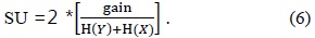
CFS algorithms are based on the concept of information theory. The FCBS algorithm developed by Yu and Liu [12] removes both irrelevant and redundant features, using SU as a goodness measure. It uses the concept of correlation based on the information theoretic concept of mutual information and entropy to calculate the uncertainty of a random variable.
Hall and Smith [3] have developed a CFS algorithm for feature selection that uses correlation to evaluate the value of features. This approach is based on the idea that good feature subsets contain features highly correlated with (predictive of) the class, yet uncorrelated with (not predictive of) each other [11]. In this algorithm, it is necessary to find the best subset from the 2
The subset generation and evaluation process terminates when it reaches the stopping criterion. Different stopping criteria are used in different algorithms. Some involve a specified limit on the number of features or a threshold value. Finally, validation data are used to validate the selected subset. In real-world applications, we do not have any prior knowledge of the relevance of a feature set. Therefore, observations are made of how changes in the feature set affect the performance of the algorithm. For example, the classification error rate or the proportion of selected features can be used as a performance indicator for a selected feature subset [8].
The adjusted Rand index, which is a clustering validation measure, has been used as a measure of correlation between the target class and a feature. Such metrics rank the features by making a comparison between the partition given by the target class and the partition of each feature [14].
General graph-theoretic clustering uses the concept of relative neighbourhood graphs [15,16]. Using the concept of neighbourliness, we define RNG(
Some clustering-based methods construct a graph using the k-nearest-neighbour approach [17]. Chameleon, which is a hierarchical clustering algorithm, uses a k-nearest-neighbour graph approach to construct a sparse graph. It then uses an algorithm to find a cluster by repeatedly combining these subclusters. Chameleon is applicable only when each cluster contains a sufficiently large number of vertices (data items).
According to Xu et al. [18], the MST clustering algorithm has been widely used. They have used this approach to represent multidimensional gene expression data. It is not pre-assumed that the data points are separated by a regular geometric curve or are grouped around centres in any MST-based clustering algorithm.
Many graph-based clustering methods take advantage of the MST approach to represent a dataset. Zhong et al. [17] employed a two-round MST-based graph representation of a dataset and developed a separated clustering algorithm and a touching clustering algorithm, encapsulating both algorithms in the same method. Zahn [19] divided a dataset into different groups according to structural features (distance, density, etc.) and captured these distinctions with different techniques. Grygorash et al. [20] proposed two algorithms using MST-based clustering algorithms. The first algorithm assumes that the number of clusters is predefined. It constructs an MST of a point set and uses an inconsistency measure to remove the edges. This process is repeated for
Shi and Malik [21] published a normalized cut criterion. Ding et al. [22] proposed a min-max clustering algorithm, in which the similarity or association between two subgraphs is minimized, while the similarity within each subgraph is maximized. It has been shown that the min-max cut leads to more balanced cuts than the ratio cut and normalized cut [21].
Our algorithm uses Kruskal’s algorithm, which is an MST-based technique of for clustering features. The clusters formed are not based on any distance or density measures. A feature is added to the cluster if it is not redundant to any of the features already present in it.
III. FEATURE SUBSET SELECTION METHOD
Entropy feature selection is a pre-processing step in many applications. Subsets are generated and then evaluated based on a heuristic. The main aim is to find the subset which has relevant and non-redundant features. In order to evaluate and classify features, we have used the information theoretic concept of information gain and entropy. Entropy is a measure of the unpredictability of a random variable. Entropy is related to the probabilities of the random variable rather than their actual values. Entropy is defined as:

Here,
If


The amount by which the entropy of

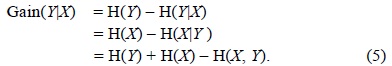
Information gain is the amount of information obtained about
Sotoca and Pla [26] have used conditional mutual information as an information theoretic measure. Conditional mutual information I(
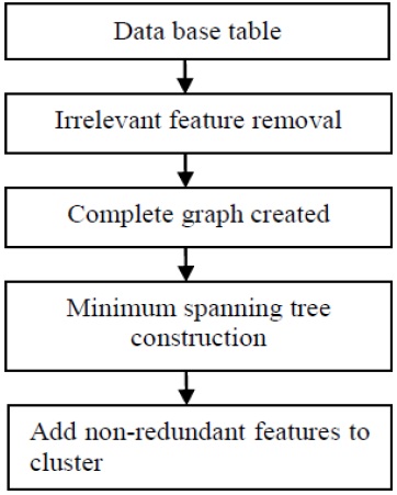
The procedure of removing irrelevant and redundant features is shown in Fig. 1.
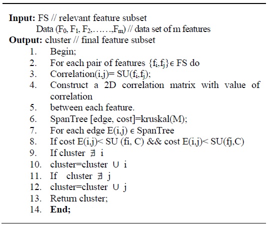
The goal of obtaining relevant features is accomplished by defining an appropriate threshold for the SU value. If the attributes from the table meet this condition, then they considered relevant and kept. Subsequently, pair-wise correlation is performed to remove redundant features and a complete weighted graph is created. An MST is then constructed. If features meet the criterion defined by the threshold value, they are added to the cluster of the feature subset, and otherwise are ignored.
Our algorithm uses the concept of SU described above to solve the problem of feature selection. It is a two-step process; first, irrelevant features are removed, and then redundant features are removed from the dataset and the final feature subset is formed.
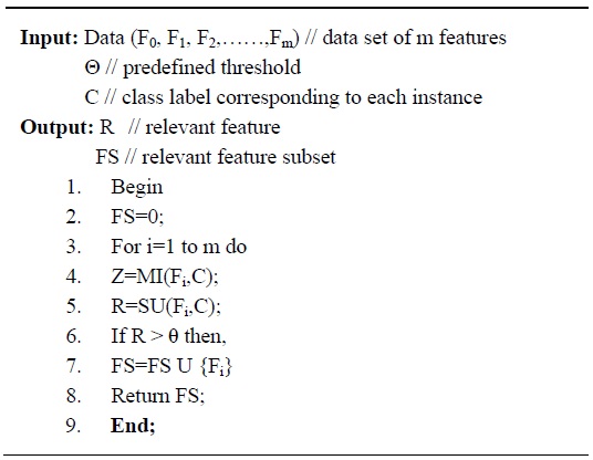
The irrelevant feature removal process evaluates whether a feature is relevant to the class or not. For each data set in Table 1, the algorithm given in Fig. 2 is applied to determine the relevant features corresponding to different threshold values. The input to this algorithm is the dataset with
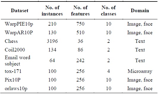
[Table 1.] Summary of data sets

Summary of data sets
Here, for the input dataset
Time Complexity: The time complexity of the method applied above is quite low. It has linear complexity and is dependent on the size of the data, as defined by the number of features and number of instances in the dataset. The time complexity is O(
In order to remove redundant features from the subset obtained above, a graph-based clustering method is applied. The vertices of the graph are the relevant features and the edges represent the correlation between two features. In order to compute the correlation among two features (
This results in a weighted complete graph with
In this section, we evaluate the performance of the algorithm described above by testing it on eight datasets of varying dimensionality, ranging from low-dimension datasets to large-dimension datasets. The ModifiedFAST algorithm was evaluated in terms of the percentage of selected features, runtime and classification accuracy.
In order to validate the proposed algorithm, eight samples of real datasets with different dimensionality were chosen from the UCI machine learning repository and from featureselection.asu.edu/datasets. The datasets contain text, microarray, or image data. The details of these datasets are described in Table 1.
Many feature selection algorithms are available in the literature. Some algorithms perform better than others with regard to individual metrics, but may perform less well from the viewpoint of other metrics.
Some classical methods used as performance metrics are:
For each dataset, we obtained the number of features after running the algorithm. Different feature selection algorithms were compared on the basis of the percentage of selected features. We then applied the naïve Bayes, the tree-based C4.5, and the rule based IB1 classification algorithms on each newly generated feature subset to calculate the classification accuracy by 10-fold cross validation.
The main target of developing a feature subset for the classification task is to improve the performance of classification algorithms. Accuracy is also the main metric for measuring classification performance. However, the number of selected features is also important in some cases.
We have developed a new performance evaluation measure resulting in a formula that integrates the number of features selected with the classification accuracy of an algorithm.
>
C. Statistical Significance Validation
Performance metrics are necessary to make observations about different classifiers. The purpose of statistical significance testing is to collect evidence representing the general behaviour of the classifiers from the results obtained by an evaluation metric. One of the tests used is the Friedman test.
The Friedman test [28] is a non-parametric approach. It can be used as a measure to compare the rank of
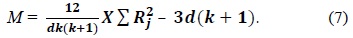
The null hypothesis of the Friedman test considered here is that there is no difference between the feature selection algorithms based on the percentage of selected features. The decision rule then states that the null hypothesis should be rejected if
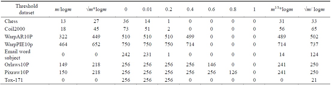
We used several threshold values in our experiment. Different feature selection algorithms, such as FCBF [12], Relief, CFS [11], and FAST [13] have likewise used different threshold values to evaluate their results. Yu and Liu [12] have suggested the relevant threshold value on SU to be the ˪m/log m˩-th ranked feature for each dataset. In FAST [13] feature selection, features are ranked by using the (√
[Table 2.] The number of relevant features found using different threshold values

The number of relevant features found using different threshold values
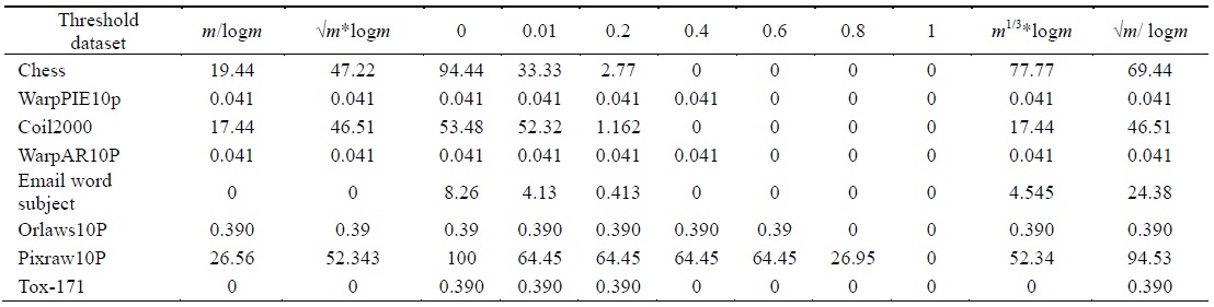
The algorithm given in Fig. 3 was applied on all the features found in Table 2 for each dataset. The final feature subset was recorded. Table 3 shows the different percentages corresponding to different thresholds. In order to choose the best thresholds for this algorithm can work, the percentage of selected features, runtime, and classification accuracy values for each threshold value were observed. Tables 4–6 record the classification accuracy along with the calculations of the proposed performance parameter
[Table 3.] Percentage of selected features using different threshold values

Percentage of selected features using different threshold values
[Table 4.] Accuracy calculated using the naive Bayes classifier
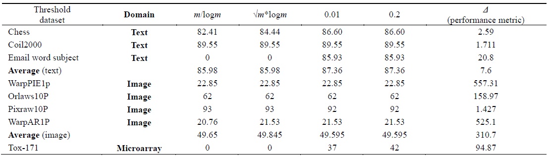
Accuracy calculated using the naive Bayes classifier
[Table 5.] Accuracy calculated using the C4.5 classifier
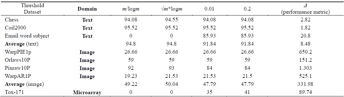
Accuracy calculated using the C4.5 classifier
[Table 6.] Accuracy calculated using the IB1 classifier
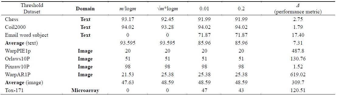
Accuracy calculated using the IB1 classifier
Tables 2–6 prove that different threshold values result in different numbers of features selected for the same dataset. In Tables 4–6, all values for each threshold have not been displayed due to space considerations. We observed experimentally that a threshold value of 0.2 yields optimal results. We also found that after feature selection, all three classifiers result in good classification accuracy for text datasets.
The datasets were categorized as low-dimension (
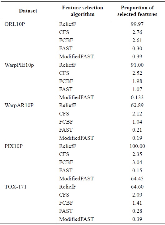
[Table 7.] Comparison of feature selection algorithms for lowdimensional datasets
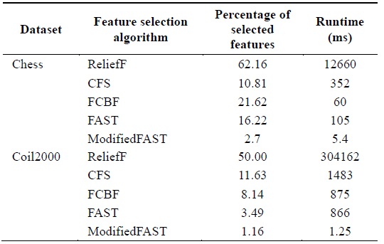
Comparison of feature selection algorithms for lowdimensional datasets
[Table 8.] Comparison of feature selection algorithms for large-dimensional datasets

Comparison of feature selection algorithms for large-dimensional datasets
When different algorithms are evaluated in terms of the percentage of features selected, we conclude that the ModifiedFAST feature selection algorithm obtains the least percentage of features in most of the datasets. This is shown in Fig. 4. ModifiedFAST yielded better results than other algorit hms in many of the datasets. The FAST algorithm took second place, followed by FCBF, CFS, and ReliefF. ModifiedFAST had the highest performance in the Chess, coil2000, WarpPIE10p, and WarpAR10P datasets. The proportion of selected features was improved in all these datasets. This shows that the optimal threshold value of 0.2 greatly improves the performance of the classification algorithms. In order to further rank the algorithms based on statistical significance, the Friedman test is used. It is used to compare
The test results falsified the null hypothesis, showing that all feature selection algorithms performed differently in terms of the percentage of selected features.
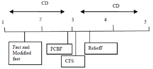
We then applied the Nemenyi test as a posthoc test [29] to explore the actual range by which pairs of algorithms differed from each other. As stated by the Nemenyi test, two classifiers are found to perform differently if the corresponding average ranks (

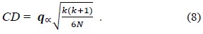
In Eq. (8),
This paper finds an optimal threshold value that can be used for most feature selection algorithms, resulting in good subsets. The thresholds given by earlier feature selection algorithms are not optimal and need to be changed. We observed that different threshold values can result in different numbers of features selected and a different level of accuracy due to changes in the number of selected features. The best threshold found for the proposed algorithm was 0.2.
We have compared the performance of the Modified FAST algorithm, based on the percentage of features selected and classification accuracy, with the values given by other feature selection algorithms, such as FAST, ReliefF, CFS, and FCBF. For text datasets, we found that the proposed algorithm resulted in improved classification accuracy than it was before the algorithm was applied for all the classifiers. On the basis of the proposed performance parameter


![Flowchart of feature selection [27].](http://oak.go.kr/repository/journal/17216/E1ICAW_2015_v13n2_113_f001.jpg)